Actor-Critic and the Credit-Assignment Dial

Dive into Deep Learning · §15.1

Actor-critic and the credit-assignment dial
bootstrap the reward-to-go · one number, two learners · the \lambda dial and its telescoping identity · bias against variance, measured

Bootstrapping the Reward-to-Go

The Monte Carlo weight waits for the episode to end. But \hat G_t = r_t + \gamma \hat G_{t+1}, and \hat V(s_{t+1}) is trained to predict exactly what \hat G_{t+1} samples. Substitute:

\delta_t = r_t + \gamma\, \hat V(s_{t+1}) - \hat V(s_t)

:eqref:eq_td_error’s scalar, with the max replaced by the policy’s own continuation.

@d2l.add_to_class(d2l.Batch)
def td_target(self, bootstrap, gamma):
    """r_t + gamma (1 - terminated) V(s'), by a numpy bootstrap."""
    return self.rew + gamma * (1 - self.term) * bootstrap(self.next_obs)

A numpy array carries no gradient graph: the target is data by construction. No detach; the boundary is the detach.

Why the TD Error Is an Advantage

If the critic were exact, \hat V = V^\pi:

E[\delta_t \mid s_t, a_t] = Q^\pi(s_t, a_t) - V^\pi(s_t).

One transition estimates what the Monte Carlo weight needed the whole remaining trajectory for.

The price: during training \hat V \ne V^\pi, so the update is biased. Variance traded for bias, the same bargain Q-learning struck, now on the policy side.

Two Learners, One Number

w \leftarrow w + \alpha_w\, \delta_t\, \nabla_w \hat V_w(s_t), \qquad \theta \leftarrow \theta + \alpha_\theta\, \delta_t\, \nabla_\theta \log \pi_\theta(a_t \mid s_t)

• the critic: sampled, bootstrapped policy evaluation; actor-critic = GPI with both halves approximate
• two-timescale intuition: the critic chases a moving target twice over, so let it learn faster; realized heuristically here as 20 fitted-TD passes (fresh target each pass), taken first

A Batched Actor-Critic: the Three-Line Diff

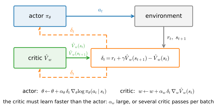
Batched episodes, one actor step per batch: a batched on-policy actor-critic, the single-environment teaching relative of A2C :cite:Mnih.Badia.Mirza.ea.2016. Against :numref:sec_deeprl’s loop, only the tail is replaced:

def train_ac(seed, ac, num_updates=num_updates):
    """The same loop with the sampled tail replaced by the bootstrap."""
    rng, env = np.random.default_rng(seed), gym.make('CartPole-v1')
    env.reset(seed=seed)
    for _ in range(num_updates):
        batch = d2l.rollout(env, ac.act, batch_episodes, rng)
        for _ in range(critic_steps):   # fresh target, one pass, repeat
            fit_value(ac, batch.obs, batch.td_target(ac.value_np, gamma))
        delta = batch.td_target(ac.value_np, gamma) - ac.value_np(batch.obs)
        gnorm = policy_step_clip(ac, batch, d2l.normalize(delta))
        yield float(batch.episode_returns().mean()), gnorm

Critic target td_target instead of G; critic_steps passes, first; weight = normalized \delta_t. Nothing else.

CartPole, Three Seeds Each

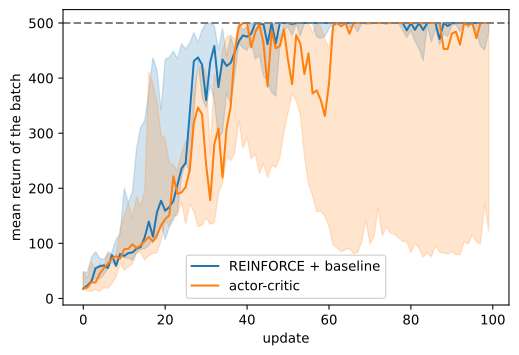
Early: actor-critic trails, the critic is still wrong. Late: both tie the 500 ceiling; only the bootstrapped side rests on it.

Not a Higher Plateau, a Still One

REINFORCE + baseline: longest stretch of perfect batches, per seed: [26, 13, 22]
        actor-critic: longest stretch of perfect batches, per seed: [39, 22, 3]

A perfect batch = all eight episodes at 500. The long streaks live on the bootstrapped side only, a run-specific stability visualization of the mechanism: the Monte Carlo weight still carries every remaining coin flip, and a run at the ceiling is one noisy batch from a stumble.

The Steps Were Never the Same Size

REINFORCE + baseline: median pre-clip gradient norm  0.03, clip binds on   0% of updates
        actor-critic: median pre-clip gradient norm  0.33, clip binds on  30% of updates

Both weights are normalized to unit variance, yet the actor-critic gradients are an order of magnitude larger: the baseline argument of :numref:sec_baselines read backwards. The state-dependent part of a weight cancels in expectation; the Monte Carlo weight spends much of its variance there, while \delta_t is almost all action-dependent signal. A better advantage estimate is a bigger step: :numref:sec_ppo.

The Critic Survives Its Moving Target

Rerun the loop, measuring both candidate weights per batch:

• \hat G_t - \hat V(s_t) = \delta_t + \gamma(\hat G_{t+1} - \hat V(s_{t+1})): one part shared signal, hundreds of parts tail
• their correlation falls from about 0.3 to zero as episodes stretch toward 500, consistent with the MC weight dissolving into tail noise (a descriptive diagnostic, not a critic certificate)
• its variance grows with the horizon; the TD error’s is pinned flat (median ratio: beyond a hundredfold)

Why survivable here: freshness keeps the critic’s training distribution matched to where its errors matter, reduced mismatch, not a guarantee (nonlinear TD can diverge even on-policy :cite:Tsitsiklis.VanRoy.1997). Our critic refreshes its target every pass, an aggressive fitted-TD loop; :numref:sec_dqn severs the freshness and reverses the choice: a frozen second copy, the target network.

The Dial

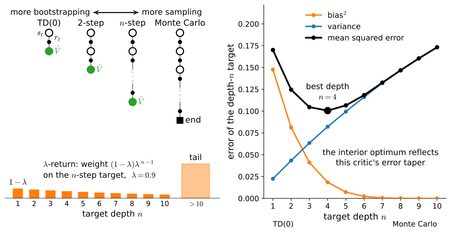
\hat G^{(n)}_t = r_t + \cdots + \gamma^{n-1} r_{t+n-1} + \gamma^n \hat V(s_{t+n}), \qquad \hat A^{\textrm{GAE}}_t = (1-\lambda) \sum_{n \ge 1} \lambda^{n-1} \big(\hat G^{(n)}_t - \hat V(s_t)\big)

Telescoping identity :cite:Schulman.Moritz.Levine.ea.2016:

\hat A^{\textrm{GAE}}_t = \sum_{l \ge 0} (\gamma\lambda)^l\, \delta_{t+l}

Each depth telescopes into TD errors; swap the sums; the inner geometric sum is \lambda^l. TD(\lambda)’s eligibility traces ran this backward, per step; streaming settings still do :cite:Elsayed.Vasan.Mahmood.2024.

GAE Is an Old Function

@d2l.add_to_class(d2l.Batch)
def gae(self, value_fn, gamma, lam):
    """GAE(gamma, lam): the reward-to-go scan, run on the TD errors."""
    delta = self.td_target(value_fn, gamma) - value_fn(self.obs)
    return self.backward_scan(delta, gamma * lam)

The reward-to-go scan of :numref:sec_baselines, run on TD errors: a new estimator is a new input to an old function.

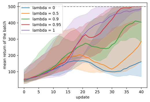
lambda = 0 is the TD error; lambda = 1 is the Monte Carlo advantage

Both endpoints asserted, not assumed.

Measuring the Dial

lambda =  0.0: best 20-update window, median 161.9, seeds [144. 145. 162. 302. 474.]
lambda =  0.5: best 20-update window, median 201.3, seeds [174. 183. 201. 312. 371.]
lambda =  0.9: best 20-update window, median 322.5, seeds [274. 319. 322. 488. 492.]
lambda = 0.95: best 20-update window, median 460.6, seeds [348. 372. 461. 486. 497.]
lambda =  1.0: best 20-update window, median 466.2, seeds [415. 456. 466. 469. 497.]

Five seeds per \lambda, a fifty-update sprint on small batches: the bottom of the dial trails decisively; from 0.9 up the arms arrive together. The sprint flatters the deep end (the critic starts ignorant); the stillness race went the other way.

Why: Bias Against Variance

lambda =  0.0: relative bias 1.34, relative variance    0.3, one-draw error    2.1
lambda =  0.5: relative bias 1.22, relative variance    0.4, one-draw error    1.9
lambda =  0.9: relative bias 0.57, relative variance    1.4, one-draw error    1.7
lambda = 0.95: relative bias 0.26, relative variance    2.4, one-draw error    2.5
lambda =  1.0: relative bias 0.00, relative variance    5.9, one-draw error    5.9

The shallow U: leaving \lambda = 1, variance collapses first and fastest; bias climbs more slowly. One-draw error is high at both pure ends, lowest strictly inside. Deployed PPO defaults commonly sit at \lambda \approx 0.9 to 0.97 (:numref:sec_ppo).

Recap

• \delta_t: a one-transition advantage estimate, unbiased only at \hat V = V^\pi; variance for bias, Q-learning’s bargain on the policy side
• the critic is sampled policy evaluation: GPI, both halves approximate, and a semi-gradient: the safety line of :numref:sec_deeprl is behind us
• batched actor-critic (A2C’s teaching relative): critic passes first, freshest critic judges
• the dial: n-step, \lambda-return, one telescoping identity, one old scan; endpoints asserted
• next: reuse the batch safely (:numref:sec_ppo, GAE by default), then sever freshness and pay (:numref:sec_dqn)