%matplotlib inline
from d2l import torch as d2l
import gymnasium as gym
import numpy as np
import torch
from torch import nn14.7 From Tables to Networks
Every algorithm in this chapter has stored what it learned in a table: sixteen rows, one per cell of the lake. Tables end where continuous states begin, because a table over real-valued coordinates has infinitely many rows and the agent will never stand in exactly the same state twice. This section makes the jump to neural networks, and its point is how little happens. The derivations of Section 14.5 and Section 14.6 never used the table: they asked for a \(\log \pi_\theta\) that is differentiable in \(\theta\), a value estimate to subtract, and a way to sample an action. We make that claim structurally rather than rhetorically: one training loop trains a network on a task no table can hold and then a Gaussian policy on a task no argmax can search, without changing a line of itself; the loop is the learned-baseline arm of Section 14.6. What is new begins with one phenomenon: generalization, an update at one state moving every other. We end the chapter by measuring it, by naming the costs that ride in with it, and by saying exactly what the resulting agent still cannot do.
%matplotlib inline
from d2l import jax as d2l
from flax import nnx
import gymnasium as gym
import jax
from jax import numpy as jnp
import numpy as np
14.7.1 Continuous States and Function Approximation
14.7.1.1 CartPole
CartPole is the classic small control problem: a cart slides along a track with a pole hinged on top, the state is four real numbers (cart position, cart velocity, pole angle, angular velocity), and the two actions push the cart left or right. Every step the pole stays up earns reward \(1\); the episode ends when the pole tips too far, the cart leaves the track, or 500 steps pass. The best possible return is therefore 500. A table over four continuous coordinates does not exist, so \(\pi_\theta\) and \(\hat{V}\) must become functions.
14.7.1.2 Replacing the Table with a Network
The ActorCritic container of Section 14.3 never asked what its policy is, only for a module that maps a state to one preference per action; .tabular happened to fill that slot with an embedding table. The constructor below fills it with a one-hidden-layer network instead, four numbers in, two preferences out, plus a second network of the same shape for the value head. The softmax of Equation 14.5.1 sits on the network’s outputs exactly as it sat on a table row; the score \(\nabla_\theta \log \pi_\theta(a \mid s)\) now carries a hidden layer’s worth of chain rule, and autograd absorbs it without a new line of ours.
@d2l.add_to_class(d2l.ActorCritic)
@classmethod
def mlp(cls, obs_dim, num_actions, hidden=64, lr=1e-2):
    """The same container with the tables replaced by one-hidden-layer nets."""
    def net(out):
        return nn.Sequential(nn.Linear(obs_dim, hidden), nn.Tanh(),
                             nn.Linear(hidden, out))
return cls(net(num_actions), net(1), lr)@d2l.add_to_class(d2l.ActorCritic)
@classmethod
def mlp(cls, obs_dim, num_actions, hidden=64, lr=1e-2, rngs=None):
"""The same container with the tables replaced by one-hidden-layer nets."""
rngs = nnx.Rngs(d2l.get_key()) if rngs is None else rngs
def net(out):
return nnx.Sequential(nnx.Linear(obs_dim, hidden, rngs=rngs), jnp.tanh,
nnx.Linear(hidden, out, rngs=rngs))
return cls(net(num_actions), net(1), lr)
_act_probs = nnx.jit(lambda net, obs: jax.nn.softmax(net(obs), -1))
@d2l.add_to_class(d2l.ActorCritic)
def act(self, obs, rng):
"""As in :numref:`sec_imitation`; the acting forward has one fixed input
shape and runs a few hundred thousand times below, so it is compiled
once and cached (:numref:`sec_compilation`)."""
if not hasattr(self, '_fwd'):
self._fwd = nnx.cached_partial(_act_probs, self.policy)
probs = np.asarray(self._fwd(jnp.asarray(obs)))
return int(rng.choice(len(probs), p=probs))The learned baseline of Section 14.6 also has to stop being a table. There, Equation 14.6.10 nudged one table entry toward the observed reward-to-go; for a network the same nudge is a regression step, mean squared error against the observed targets, run through the optimizer the container already owns. The num_steps argument sets how many regression steps the critic takes per batch; this section leaves the knob at \(1\), and Section 15.1 turns it.
def fit_value(ac, obs, target, num_steps=1):
    """Regress the value head on a fixed target: eq_value_baseline for nets."""
    obs, target = torch.as_tensor(obs), torch.as_tensor(target)
    for _ in range(num_steps):
        loss = ((ac.V(obs) - target) ** 2).mean()
        ac.opt_v.zero_grad()
        loss.backward()
        ac.opt_v.step()
    return loss.item()
def fit_value(ac, obs, target, num_steps=1):
"""Regress the value head on a fixed target: eq_value_baseline for nets.
Not jitted: batches change shape at every update; jit would recompile."""
obs, target = jnp.asarray(obs), jnp.asarray(target)
for _ in range(num_steps):
loss, grads = nnx.value_and_grad(
lambda value: ((ac.V(obs, value) - target) ** 2).mean())(ac.value)
ac.opt_v.update(ac.value, grads)
return float(loss)Now the training function, and it is the reason this section exists. It is the learned-baseline arm of Section 14.6 line for line (rollout, reward_to_go, a weight, policy_step, the value update), with the arm frozen and two things promoted to arguments, the constructor and the environment, because the whole point is to hand it different ones. The weight line joins the ladder’s last two rungs: the learned baseline gives each weight its zero point, and normalize rescales the batch, which Section 14.6 identified as a per-batch step size; we keep it because this one function is about to train on tasks whose returns differ by two orders of magnitude, and no single learning rate serves both scales unaided. One deliberate reversal: that section raced its arms under plain SGD so that no adaptive optimizer would absorb the scale effects it was measuring. That was a measurement choice, not a recommendation; for training networks Adam is the right tool, and the choice lives where it belongs, inside the policy object whose constructor owns its optimizers rather than in the algorithm.
def train_reinforce(seed, make_agent, env_name, gamma=0.99, num_updates=80,
                    batch_episodes=8):
    """The learned-baseline REINFORCE of :numref:`sec_baselines`, unchanged;
    what varies is the policy object handed in by `make_agent`."""
    rng, env = np.random.default_rng(seed), gym.make(env_name)
    ac = make_agent(seed)
    env.reset(seed=seed)
    for _ in range(num_updates):
        batch = d2l.rollout(env, ac.act, batch_episodes, rng)
        G = batch.reward_to_go(gamma)
        w = d2l.normalize(G - ac.value_np(batch.obs))
        L = d2l.policy_step(ac, batch, w)
        fit_value(ac, batch.obs, G)
        yield float(batch.episode_returns().mean()), L
def train_reinforce(seed, make_agent, env_name, gamma=0.99, num_updates=80,
batch_episodes=8):
"""The learned-baseline REINFORCE of :numref:`sec_baselines`, unchanged;
what varies is the policy object handed in by `make_agent`."""
rng, env = np.random.default_rng(seed), gym.make(env_name)
ac = make_agent(seed)
env.reset(seed=seed)
for _ in range(num_updates):
batch = d2l.rollout(env, ac.act, batch_episodes, rng)
G = batch.reward_to_go(gamma)
w = d2l.normalize(G - ac.value_np(batch.obs))
L = d2l.policy_step(ac, batch, w)
fit_value(ac, batch.obs, G)
yield float(batch.episode_returns().mean()), LAgainst Section 14.6, the diff that moves this loop from the lake to the cart is three lines long: the constructor is ActorCritic.mlp(4, 2) instead of ActorCritic.tabular(16, 4), the environment is 'CartPole-v1' instead of 'FrozenLake-v1', and the discount is \(0.99\), suited to a 500-step horizon, instead of \(0.95\). Nothing else. Three seeds:
if tab.selected('pytorch'):
    def cartpole_agent(seed):
        torch.manual_seed(seed)
        return d2l.ActorCritic.mlp(4, 2)
if tab.selected('jax'):
    def cartpole_agent(seed):
        return d2l.ActorCritic.mlp(4, 2, rngs=nnx.Rngs(seed))

runs = d2l.run_seeds(train_reinforce, 3, make_agent=cartpole_agent,
                     env_name='CartPole-v1')
d2l.plot_curves({'REINFORCE + learned baseline': runs[:, :, 0]},
                xlabel='update', ylabel='mean return of the batch',
                reference=500)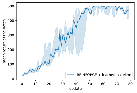
if tab.selected('pytorch'):
    def cartpole_agent(seed):
        torch.manual_seed(seed)
        return d2l.ActorCritic.mlp(4, 2)
if tab.selected('jax'):
    def cartpole_agent(seed):
        return d2l.ActorCritic.mlp(4, 2, rngs=nnx.Rngs(seed))

runs = d2l.run_seeds(train_reinforce, 3, make_agent=cartpole_agent,
                     env_name='CartPole-v1')
d2l.plot_curves({'REINFORCE + learned baseline': runs[:, :, 0]},
                xlabel='update', ylabel='mean return of the batch',
                reference=500)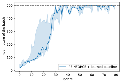
The curve climbs from about 20, the return of the untrained random policy, to the ceiling’s neighborhood: every seed’s per-update batch mean crosses 400 within about fifty updates and holds above 400 to the end. Where in that upper range a seed settles moves from run to run, so read the level and not the last digit. The tabular derivation survived the move without a single new equation.
14.7.1.3 Tables as Linear Networks on One-Hot States
The swap is small because it is not really a swap. ActorCritic.tabular stores its preferences in an embedding table, and an embedding is a linear layer applied to one-hot inputs: selecting row \(s\) of a \(16 \times 4\) table is multiplying the table’s transpose by the indicator vector of \(s\). Every “tabular” method in this chapter was therefore already training a network, the smallest possible one, a single linear map with no bias under a fixed one-hot feature map. What changed today is only the features. One-hot features are mutually orthogonal, so no two states share a single parameter, and an update at one state cannot touch any other; the hidden layer makes features overlap, and overlapping features are what generalization means. That difference, not depth and not width, is the first thing networks change about reinforcement learning and the one this section can measure; the rest of the bill (nonconvex optimization, extrapolation error where the data thins out, and interference between updates) rides in with the shared parameters and comes due in Chapter 15.
14.7.2 Continuous Actions and Stochastic Policies
14.7.2.1 The Gaussian Policy
Pendulum is the smallest task whose actions are continuous: a pendulum hangs from a motorized pivot, the state is \((\cos\vartheta, \sin\vartheta, \dot\vartheta)\), and the action is a torque in \([-2, 2]\). The reward is never positive, each step charges roughly the squared angle from upright plus small penalties on speed and torque, and an episode lasts 200 steps, so a policy that spins aimlessly collects about \(-1200\) per episode while a controller that swings up and balances collects about \(-200\). The torque is one real number, so a softmax over actions is not available even in principle.
The fix costs fifteen lines. Let the network emit the mean of the action, keep one learned parameter for its log standard deviation, and let the policy be the Gaussian \(\pi_\theta(a \mid s) = \mathcal{N}\big(a;\, \mu_\theta(s), \sigma^2\big)\). GaussianPolicy subclasses ActorCritic and overrides exactly the three methods that define what kind of distribution the policy is: log_prob, act, and act_greedy. Everything that consumes the policy (rollout, policy_step, fit_value, train_reinforce) touches only that interface, so none of it can even tell. The log standard deviation lives inside the policy head, not on the container, so that policy_step, which differentiates the policy module, cannot miss it.
class GaussianHead(nn.Module):
    """Mean network plus a state-independent learned log standard deviation."""
    def __init__(self, obs_dim, act_dim, hidden):
        super().__init__()
        self.mean = nn.Sequential(nn.Linear(obs_dim, hidden), nn.Tanh(),
                                  nn.Linear(hidden, act_dim))
        self.log_std = nn.Parameter(torch.zeros(act_dim))

    def forward(self, obs):
        return self.mean(obs), self.log_std.exp()

class GaussianPolicy(d2l.ActorCritic):
    """The same interface over a Normal instead of a softmax; nothing that
    consumes the interface changes."""
    def __init__(self, obs_dim, act_dim, hidden=64, lr=1e-2):
        super().__init__(GaussianHead(obs_dim, act_dim, hidden),
                         nn.Sequential(nn.Linear(obs_dim, hidden), nn.Tanh(),
                                       nn.Linear(hidden, 1)), lr)

    def log_prob(self, obs, act):
        mean, std = self.policy(obs)
        return torch.distributions.Normal(mean, std).log_prob(act).sum(-1)

    def act(self, obs, rng):
        with torch.no_grad():
            mean, std = self.policy(torch.as_tensor(obs))
        return mean.numpy() + std.numpy() * rng.standard_normal(
            mean.shape, dtype=np.float32)

    def act_greedy(self, obs, rng=None):
        with torch.no_grad():
            return self.policy(torch.as_tensor(obs))[0].numpy()
class GaussianHead(nnx.Module):
"""Mean network plus a state-independent learned log standard deviation."""
def __init__(self, obs_dim, act_dim, hidden, rngs):
self.mean = nnx.Sequential(nnx.Linear(obs_dim, hidden, rngs=rngs),
jnp.tanh,
nnx.Linear(hidden, act_dim, rngs=rngs))
self.log_std = nnx.Param(jnp.zeros(act_dim))
def __call__(self, obs):
return self.mean(obs), jnp.exp(self.log_std[...])
class GaussianPolicy(d2l.ActorCritic):
"""The same interface over a Normal instead of a softmax; nothing that
consumes the interface changes."""
def __init__(self, obs_dim, act_dim, hidden=64, lr=1e-2, rngs=None):
rngs = nnx.Rngs(d2l.get_key()) if rngs is None else rngs
super().__init__(GaussianHead(obs_dim, act_dim, hidden, rngs),
nnx.Sequential(nnx.Linear(obs_dim, hidden, rngs=rngs),
jnp.tanh,
nnx.Linear(hidden, 1, rngs=rngs)), lr)
def log_prob(self, obs, act, policy=None):
mean, std = (self.policy if policy is None else policy)(obs)
return jax.scipy.stats.norm.logpdf(act, mean, std).sum(-1)
def act(self, obs, rng):
if not hasattr(self, '_fwd'): # compile the fixed-shape acting
self._fwd = nnx.cached_partial(nnx.jit(lambda net, o: net(o)),
self.policy) # forward, once
mean, std = self._fwd(jnp.asarray(obs))
return np.asarray(mean) + np.asarray(std) * rng.standard_normal(
mean.shape, dtype=np.float32)
def act_greedy(self, obs, rng=None):
return np.asarray(self.policy(jnp.asarray(obs))[0])The environment clips whatever torque the sample lands on to \([-2, 2]\), so act may return the raw draw. Before trusting the new log_prob inside a training run, we check it the way Section 14.5 checked the softmax score, against the density written by hand; at initialization \(\sigma = e^0 = 1\), so the handwritten Gaussian needs only the mean, which act_greedy reads out:
if tab.selected('pytorch'):
    torch.manual_seed(1)
    gp = GaussianPolicy(3, 1)
if tab.selected('jax'):
    gp = GaussianPolicy(3, 1, rngs=nnx.Rngs(1))
rng = np.random.default_rng(1)
obs = rng.standard_normal((5, 3)).astype(np.float32)
act = rng.standard_normal((5, 1)).astype(np.float32)
mean = np.stack([gp.act_greedy(o) for o in obs])
hand = -0.5 * (act - mean) ** 2 - 0.5 * np.log(2 * np.pi)
print(np.allclose(gp.log_prob_np(obs, act), hand.sum(-1), atol=1e-5))Trueif tab.selected('pytorch'):
torch.manual_seed(1)
gp = GaussianPolicy(3, 1)
if tab.selected('jax'):
gp = GaussianPolicy(3, 1, rngs=nnx.Rngs(1))
rng = np.random.default_rng(1)
obs = rng.standard_normal((5, 3)).astype(np.float32)
act = rng.standard_normal((5, 1)).astype(np.float32)
mean = np.stack([gp.act_greedy(o) for o in obs])
hand = -0.5 * (act - mean) ** 2 - 0.5 * np.log(2 * np.pi)
print(np.allclose(gp.log_prob_np(obs, act), hand.sum(-1), atol=1e-5))True14.7.2.2 The Score Function with Continuous Actions
Why does the same estimator apply? Look back at the derivation of Equation 14.5.6: the log-derivative trick asked only that \(\log \pi_\theta\) be differentiable in \(\theta\), and the sum over trajectories became an expectation that sampling estimates. Nowhere did it enumerate the action set. For the Gaussian, \(\nabla_\theta \log \pi_\theta(a \mid s)\) is as available as it was for the softmax, so REINFORCE with a learned baseline runs on Pendulum through the identical training path. The function does not change; its arguments do. The task is harder (the agent must discover swinging up before holding still can pay), so it gets more updates; and it gets a shorter credit horizon, \(\gamma = 0.95\), because with a cost arriving at every one of 200 steps, a wide discount window buries the consequences of a single torque under a hundred steps of unrelated future. Be clear about what that knob is: the discount is part of the objective (Section 14.1), so choosing \(\gamma = 0.95\) redefines what is being maximized, trading long-horizon credit for a learnable signal; it is a design decision about the task, not a free estimator setting:
if tab.selected('pytorch'):
    def pendulum_agent(seed):
        torch.manual_seed(seed)
        return GaussianPolicy(3, 1)
if tab.selected('jax'):
    def pendulum_agent(seed):
        return GaussianPolicy(3, 1, rngs=nnx.Rngs(seed))

runs_p = d2l.run_seeds(train_reinforce, 3, make_agent=pendulum_agent,
                       env_name='Pendulum-v1', gamma=0.95, num_updates=300)
d2l.plot_curves({'REINFORCE + learned baseline': runs_p[:, :, 0]},
                xlabel='update', ylabel='mean return of the batch',
                reference=-200, smooth=10)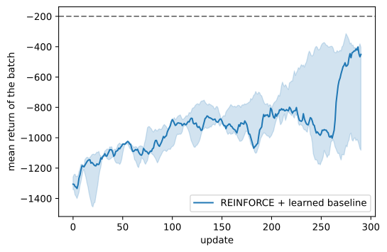
if tab.selected('pytorch'):
    def pendulum_agent(seed):
        torch.manual_seed(seed)
        return GaussianPolicy(3, 1)
if tab.selected('jax'):
    def pendulum_agent(seed):
        return GaussianPolicy(3, 1, rngs=nnx.Rngs(seed))

runs_p = d2l.run_seeds(train_reinforce, 3, make_agent=pendulum_agent,
                       env_name='Pendulum-v1', gamma=0.95, num_updates=300)
d2l.plot_curves({'REINFORCE + learned baseline': runs_p[:, :, 0]},
                xlabel='update', ylabel='mean return of the batch',
                reference=-200, smooth=10)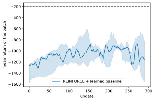
The curve starts between the \(-1200\) and \(-1600\) of an aimless policy and climbs: at the best stretch of its run, each seed has cut its starting cost by somewhere between a quarter and three quarters, depending on seed and framework. Two observations temper the celebration, and both are data. No seed reaches the dashed line at \(-200\), the neighborhood of a controller that swings up and holds: REINFORCE pays for every improvement with fresh episodes, and this task sits near the edge of what that bill can buy at textbook scale. And the gains are not always kept: under a fixed step size the policy keeps moving, and a seed can give back much of its progress before the run ends, a failure the end of this chapter names and Section 15.2 repairs. So we claim improvement, not mastery, and the improvement is the point: a continuous-action policy trained through a function that does not know the word continuous. One more reading of the same object is worth a sentence: a language model is this policy’s discrete twin, a network mapping a state (the context) to a distribution over actions (the vocabulary), and the updates that tune one at scale are the updates that just ran (Section 15.7).
14.7.2.3 Score-Function versus Pathwise Gradients
There is a second way to differentiate an expected value, and seeing both on one problem explains a fault line that runs through all of deep reinforcement learning. Take a single state, a Gaussian policy \(a \sim \mathcal{N}(\mu, \sigma^2)\), and a known, differentiable reward \(Q(a)\). The gradient of \(E[Q(a)]\) with respect to \(\mu\) can be written two ways,
\[\nabla_\mu\, E\big[ Q(a) \big] = E\Big[ Q(a)\, \frac{a - \mu}{\sigma^2} \Big] = E\big[ Q'(\mu + \sigma z) \big], \qquad z \sim \mathcal{N}(0, 1). \tag{14.7.1}\]
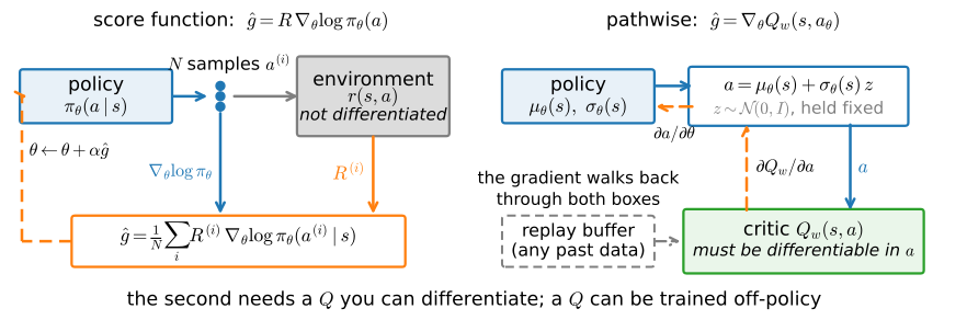
The first equality is the score-function identity this chapter is built on. The second substitutes \(a = \mu + \sigma z\), so that \(\mu\) appears inside \(Q\) rather than inside the distribution, and differentiates straight through the sample; it is the pathwise or reparameterization gradient (Kingma and Welling 2014), and Figure 14.7.1 draws where each estimator’s gradient flows. Both are unbiased. They are not equally noisy:
def Q(a):                     # a stand-in critic, differentiable in the action
    return -(a - 1.0) ** 2

sigma, N = 0.5, 100000
a = sigma * np.random.default_rng(2).standard_normal(N, dtype=np.float32)
g_score = Q(a) * a / sigma ** 2               # score-function samples, mu = 0
at = torch.as_tensor(a).requires_grad_(True)  # pathwise: grad through a
Q(at).sum().backward()
g_path = at.grad.numpy()                      # per-sample dQ/da (da/dmu = 1)
print(f'score:    mean {g_score.mean():.2f}, variance {g_score.var():.1f}')
print(f'pathwise: mean {g_path.mean():.2f}, variance {g_path.var():.2f}')
print(f'score variance if Q gains a constant +10: '
      f'{((Q(a) + 10) * a / sigma ** 2).var():.0f}; pathwise is unchanged')
score: mean 1.98, variance 21.5
pathwise: mean 2.00, variance 1.00
score variance if Q gains a constant +10: 281; pathwise is unchangeddef Q(a): # a stand-in critic, differentiable in the action
return -(a - 1.0) ** 2
sigma, N = 0.5, 100000
a = sigma * np.random.default_rng(2).standard_normal(N, dtype=np.float32)
g_score = Q(a) * a / sigma ** 2 # score-function samples, mu = 0
g_path = np.asarray(jax.vmap(jax.grad(Q))(jnp.asarray(a))) # per-sample dQ/da
print(f'score: mean {g_score.mean():.2f}, variance {g_score.var():.1f}')
print(f'pathwise: mean {g_path.mean():.2f}, variance {g_path.var():.2f}')
print(f'score variance if Q gains a constant +10: '
f'{((Q(a) + 10) * a / sigma ** 2).var():.0f}; pathwise is unchanged')score: mean 1.98, variance 21.5
pathwise: mean 2.00, variance 1.00
score variance if Q gains a constant +10: 281; pathwise is unchangedBoth means sit at the exact gradient of \(2.0\). The variances differ by a factor of about twenty, and the last line shows why the gap is structural rather than incidental: add a constant to every reward and the score estimator’s variance explodes by another order of magnitude, because the score only ever sees \(Q\) as a scalar weight, which is precisely the noise Section 14.6 spent a section subtracting away. The pathwise estimator never sees the constant at all, since it consumes \(Q\) only through the derivative \(Q'\). Its price is in the premise: it needs \(Q\) as a differentiable function of the action, not just sampled returns.
14.7.2.4 The Argmax over Continuous Actions
One casualty of the continuous action deserves its own account. Every value-based method in this chapter extracted its policy by an argmax over actions: value_iteration maximized over four entries, q_learning’s target contained \(\max_{a'} Q(s', a')\), epsilon_greedy argmaxed a row. Over four actions that is a table lookup; over \(a \in \mathbb{R}^d\) it is an optimization problem in its own right, to be solved at every environment step and inside every update target, and the value family dies of it: this is why Section 15.4 will keep its actions discrete. The policy methods never noticed the funeral, because sampling replaced enumeration.
The standard continuous-action answer for the value family is to train a second network to be the argmax: a deterministic policy trained to output the action that maximizes a learned critic \(Q_w(s, a)\), whose training signal is exactly the pathwise gradient \(\partial Q_w / \partial a \cdot \partial a / \partial \theta\) of Figure 14.7.1. Two independent axes now sort the algorithm landscape, and their independence is the point. One axis is the gradient estimator, score function or pathwise. The other is the data allowed to drive the update, on-policy or off-policy. The pathwise route pairs naturally with off-policy data, because its critic is trained by regression and regression accepts transitions from anywhere, a replay buffer included; but the pairing is an affinity, not an implication. A score-function estimator can be corrected for off-policy data with the importance ratios of Section 15.2, and a pathwise method still needs its buffer to cover the states and actions the current policy visits. Nor does the pathwise axis force determinism: DDPG and TD3 are deterministic actor-critic methods, while SAC trains a stochastic actor by the same reparameterized gradient, entropy-regularized and off-policy. What is true is the practical clustering: the off-policy continuous-control family (DDPG, TD3, SAC) is built around a pathwise gradient through an action-differentiable critic and reuses every transition many times, while the score-function methods (REINFORCE today, actor-critic and PPO in Chapter 15) run on-policy, paying for a fresh batch per update as Section 14.5 priced it. When a practitioner asks “PPO or SAC?”, the two axes are the content of the question: which gradient estimator, and which data may drive the update.
14.7.3 Generalization across States
14.7.3.1 Measuring State Coupling
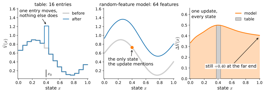
The move to networks did change something, and it is not the mathematics. A table update touches one row; a network update touches every state at once, because all states share the same weights. Figure 14.7.2 draws the claim, and it is measurable in eight lines: take a value head over a cloud of 256 random states, ask fit_value to raise its estimate at one of them by one unit, and watch what happens everywhere else. Then file the same request against the tabular container.
if tab.selected('pytorch'):
    torch.manual_seed(0)
    net_probe, tab_probe = d2l.ActorCritic.mlp(4, 2), \
        d2l.ActorCritic.tabular(16, 4)
if tab.selected('jax'):
    net_probe = d2l.ActorCritic.mlp(4, 2, rngs=nnx.Rngs(0))
    tab_probe = d2l.ActorCritic.tabular(16, 4, rngs=nnx.Rngs(0))
S = np.random.default_rng(0).uniform(-1, 1, (256, 4)).astype(np.float32)
before = net_probe.value_np(S)
fit_value(net_probe, S[:1], before[:1] + 1.0, num_steps=25)   # raise ONE state
dV = net_probe.value_np(S) - before
before_t = tab_probe.value_np(np.arange(16))
fit_value(tab_probe, np.arange(1), before_t[:1] + 1.0, num_steps=25)
dV_t = tab_probe.value_np(np.arange(16)) - before_t
print(f'network: nudged state moved {dV[0]:+.2f}; '
      f'{(np.abs(dV[1:]) > 1e-4).sum()} of the 255 others moved too, '
      f'|change| up to {np.abs(dV[1:]).max():.2f}')
print(f'table:   nudged entry moved {dV_t[0]:+.2f}; '
      f'largest move among the other fifteen: {np.abs(dV_t[1:]).max():.6f}')
network: nudged state moved +1.16; 255 of the 255 others moved too, |change| up to 1.19
table: nudged entry moved +1.18; largest move among the other fifteen: 0.000000if tab.selected('pytorch'):
torch.manual_seed(0)
net_probe, tab_probe = d2l.ActorCritic.mlp(4, 2), \
d2l.ActorCritic.tabular(16, 4)
if tab.selected('jax'):
net_probe = d2l.ActorCritic.mlp(4, 2, rngs=nnx.Rngs(0))
tab_probe = d2l.ActorCritic.tabular(16, 4, rngs=nnx.Rngs(0))
S = np.random.default_rng(0).uniform(-1, 1, (256, 4)).astype(np.float32)
before = net_probe.value_np(S)
fit_value(net_probe, S[:1], before[:1] + 1.0, num_steps=25) # raise ONE state
dV = net_probe.value_np(S) - before
before_t = tab_probe.value_np(np.arange(16))
fit_value(tab_probe, np.arange(1), before_t[:1] + 1.0, num_steps=25)
dV_t = tab_probe.value_np(np.arange(16)) - before_t
print(f'network: nudged state moved {dV[0]:+.2f}; '
f'{(np.abs(dV[1:]) > 1e-4).sum()} of the 255 others moved too, '
f'|change| up to {np.abs(dV[1:]).max():.2f}')
print(f'table: nudged entry moved {dV_t[0]:+.2f}; '
f'largest move among the other fifteen: {np.abs(dV_t[1:]).max():.6f}')network: nudged state moved +1.12; 255 of the 255 others moved too, |change| up to 1.20
table: nudged entry moved +1.18; largest move among the other fifteen: 0.000000The network grants the request and bills every other state for it: all 255 states we never mentioned move, some by as much as the request itself. The table moves one entry and nothing else, to the sixth decimal place. Neither behavior is the good one. Generalization is why CartPole was learnable at all: the agent visited on the order of a hundred thousand states it can never see again, and only weight sharing lets one of them teach another. And generalization is why the training curve dips on its way up: an update driven by one batch moves the policy and the values at every state, including states the batch never visited, for better and for worse. Tables never did that. The coupling returns as a central difficulty when value functions are trained by bootstrapping in Section 15.4.
14.7.3.2 Why Policy Gradients Survive Function Approximation
It is worth being precise about why the swap was safe, because the reason draws the boundary between this chapter and the next. A policy-gradient update estimates the gradient of a fixed, stationary scalar objective \(J(\theta)\) (Equation 14.5.4), and Section 14.5 checked the estimator’s mean against that gradient. That is the shape of stochastic gradient ascent, and the guarantees of Section 9.3 attach to that shape under their usual conditions (smoothness, unbiased estimates of bounded variance, decaying step sizes); our loop does not meet them to the letter, since normalize rescales each batch by a data-dependent factor, the batches are correlated with the policy that collected them, and Adam runs at a fixed step, so the curves above are evidence about these runs rather than instances of a theorem. What the loop does keep is the structural safeguard: neither update chases its own output. The critic here is supervised regression on targets computed from data, reward-to-go values that do not contain the critic’s own predictions. The moment a value function’s targets are built from the value function itself, bootstrapping, that safeguard is gone, and the failure deserves a precise name: each individual update, target held fixed, is still a legitimate gradient step on a regression loss, but the expected update direction, the semi-gradient field, is generally not the gradient of any single scalar objective; its fixed point is defined by self-consistency rather than by minimizing anything, and with function approximation in the loop the iteration can diverge outright (Tsitsiklis and Van Roy 1997). (The residual-gradient alternative descends the Bellman error itself and restores a true objective, at the price of the double-sampling problem of Section 14.4, which is why it is rarely preferred.) Everything in this section stayed on the safe side of that line. Chapter 15 steps over it in its first section, and Section 15.4 is about what it costs.
14.7.4 The Surrogate Loss
One implementation habit deserves a closing word, because every framework codebase you will read is organized around it. Deep learning frameworks want a loss to minimize, so instead of assembling the estimator \(\hat{u}\) of Section 14.6 by hand, we write the scalar
\[L(\theta) = -\frac{1}{N} \sum_{\textrm{steps}} \hat{A}_t\, \log \pi_\theta(a_t \mid s_t), \tag{14.7.2}\]
with the advantages \(\hat{A}_t\) treated as fixed numbers. Its gradient is \(-\hat{u}\) up to a positive per-batch factor (the batch’s mean episode length, the step-averaging choice Section 14.6 catalogued), so one optimizer step on \(L\) is one gradient ascent step on the return. This is exactly what policy_step has computed since Section 14.3, and “treated as fixed” is enforced there by construction: the weights arrive as a numpy array, which cannot carry a gradient graph. New at network scale is only the temptation to read the number, because every other loss in this book was worth reading. This one is not: \(L\) is a scalar whose derivative equals the estimator, nothing more. The value of \(L\) itself means nothing; a falling loss does not indicate progress here, only the return curve does. The CartPole runs already logged \(L\) beside the return, so the claim is one plot away:
d2l.plot_curves({'CartPole': runs[:, :, 1]}, xlabel='update',
                ylabel='policy loss L')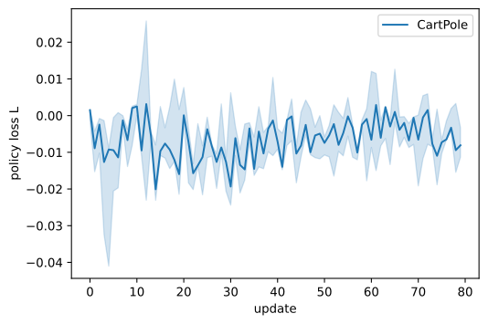
d2l.plot_curves({'CartPole': runs[:, :, 1]}, xlabel='update',
                ylabel='policy loss L')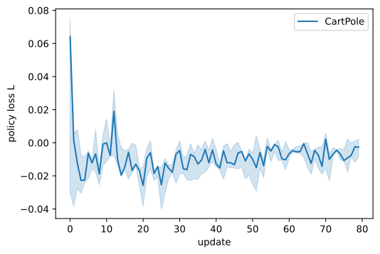
Set this against the return curve above it: while the return climbed twenty-fold, the loss wandered around zero with no trend that survives across seeds, exactly as it should, since the normalized advantages average to zero by construction and \(L\) measures nothing but their momentary correlation with the log-probabilities. An engineer watching this panel and expecting descent would conclude the run is broken while the agent quietly masters the task. In Chapter 15 the same lesson recurs one level up: what is worth watching are diagnostics of the update (ratios, divergences, entropies), never the loss.
That closes the chapter, and it is worth stating plainly what the agent we now have cannot do. It waits for episodes to end before it learns anything, because its critic regresses on complete reward-to-go sums; Section 15.1 bootstraps instead, buying updates mid-episode at the price of bias. It throws every batch away after one gradient step, the on-policy bill Section 14.5 priced; Section 15.2 makes reuse safe, and Section 15.4 rebuilds learning around a buffer of old experience. And nobody has told it how big a step is safe: a policy, unlike a regression fit, generates its own future data, so one over-large step can destroy the very distribution it must learn from next; pricing that step is Section 15.2’s subject. Those three debts, in that order, are Chapter 15.
14.7.5 Summary
Tables hold one number per state, so they cannot represent a policy or a value over continuous states; but a table was only ever the smallest network, a linear map on one-hot features, so the algorithms of this chapter never depended on it. ActorCritic.mlp swaps the embedding for a one-hidden-layer network, fit_value restates the value-baseline update Equation 14.6.10 as regression, and the learned-baseline REINFORCE of Section 14.6 trains CartPole to near its 500 ceiling unchanged. A Gaussian head extends the same interface to continuous actions, where the argmax of the value family has no meaning, and the same training function improves Pendulum. The score-function and pathwise gradients estimate the same derivative at very different variances, and two independent axes sort the landscape: the estimator (score or pathwise) and the data (on- or off-policy). Their practical pairing (pathwise gradients with replayed data in DDPG, TD3 and the stochastic-actor SAC, against score functions with fresh batches in the PPO family) is an affinity, not an implication. What networks most visibly change is generalization: one update moves every state, which is why continuous tasks are learnable and why training curves dip. Policy-gradient updates remained estimates of the gradient of one stationary objective throughout; bootstrapped value learning, whose expected update is generally the gradient of nothing, begins in Chapter 15.
What the experiments show, and what they do not. All curves come from three seeded runs per task through one shared training function, sampling through one numpy stream per run; the two framework tabs share every batch-collection line but initialize their networks from different distributions, so their curves differ seed by seed while supporting the same statements. On CartPole, every seed’s per-update batch mean crosses 400 within about fifty updates and stays above 400. On Pendulum, every seed’s best stretch lands somewhere between about \(-300\) and \(-900\) from starts of \(-1200\) to \(-1600\), no seed approaches \(-200\), and the framework tabs disagree more than they do on CartPole, exactly what wide seed spread on an unstable task predicts; the prose therefore claims only what all runs share: improvement without mastery. The policy loss carries no signal about either task. The nudge measurement and the variance comparison are deterministic probes, and the factor-twenty gap between the score and pathwise variances is specific to this \(Q\), this \(\sigma\), and this constant offset, though its direction and its mechanism are not. Following Section 14.6’s own advice, three seeds license trends, levels, and orderings, never digits. The compute belongs to readers.
14.7.6 Exercises
- [conceptual] A loss that is not a loss. Show that the gradient of Equation 14.7.2 equals \(-\hat{u}\) up to a positive constant when the advantages are held fixed. Then describe a situation in which the value of that loss decreases while the return also decreases, and say what you should plot instead.
- [short-code] How small can the policy be. Sweep the hidden width over \(\{4, 16, 64\}\), two seeds each, and report the mean return over the last ten updates. How small can the network be and still balance the pole, and what changes about the speed and the smoothness of training at each end? (About ten minutes on a laptop CPU.)
- [short-code] Which return to plot.
train_reinforcereports the undiscounted episode return but uses discounted reward-to-go inside the update. Add the discounted return to the plot. Why do the two tell the same story here, and construct a task where they would not. - [short-code] Batch size at a fixed episode budget. Sweep the batch size over \(\{1, 8, 32\}\) with the total number of sampled episodes held fixed, so that smaller batches take proportionally more updates. Which end learns fastest per episode, and which gives the smoothest curve? Which of the two would you optimize if episodes were expensive?
- [short-code] Advantage scale. Replace the normalized advantage in
train_reinforceby the raw reward-to-go, as in Section 14.5, and rerun both tasks. Which of the two tasks degrades more, and why? (Compare the typical magnitude of \(\hat{G}_t\) on CartPole and on Pendulum, and recall which optimizer the policy uses.) - [conceptual] Generalization cuts both ways. On FrozenLake an update touched one row of a table. Here it moves the policy at every state at once. Argue why a batch dominated by near-vertical-pole states can make the policy worse at large pole angles, and name two phenomena in Chapter 15 that are consequences of the same coupling.
- [short-code] What the spread costs. Fix the Gaussian head’s
log_std(delete the parameter and hard-code \(\sigma\)) at each of \(\sigma \in \{0.1, 1.0, 4.0\}\) and rerun Pendulum with two seeds each. What does an over-small \(\sigma\) cost, and what does an over-large one cost? Relate the two failures to exploration and to the score’s variance in Equation 14.7.1, and note what the environment’s torque clip at \(\pm 2\) does to the largest choice.