%matplotlib inline
from d2l import torch as d2l
import gymnasium as gym
import numpy as np14.1 Markov Decision Processes
Everywhere else in this book, a model’s prediction changes nothing about the data it is shown next. An agent that acts has no such luxury: press a key, and the world that answers is the world the keypress created. Learning to act therefore needs a model of acting itself. The Markov decision process (MDP) (Bellman 1957; Puterman 1994) is that model: four objects and one assumption that turn “act well over time” into a mathematical problem.
We build the object twice: first as data read out of a running simulator, then as notation, because notation is easier to trust once printed. Three of the four objects are facts about the world. The fourth, the reward, is written by you, and the section’s final experiment shows an optimizer doing exactly what a plausible reward says instead of what its author meant. Our laboratory is a frozen lake of sixteen cells whose ice does not respect commands.
%matplotlib inline
from d2l import jax as d2l
import gymnasium as gym
import numpy as np
14.1.1 The Model
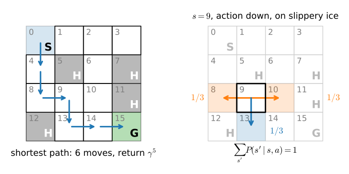
Figure 14.1.1 shows the environment that carries the next four sections: FrozenLake, from the Gymnasium suite (Towers et al. 2024). The agent starts at the top-left cell and wants the goal at the bottom right, which pays a reward of one; four cells are holes; reaching either ends the episode. The rest is slippery ice: a commanded move goes as intended with probability \(1/3\) and slides to one of the two perpendicular neighbors with probability \(1/3\) each. Commands are proposals, not guarantees.
14.1.1.1 States, Actions and the Transition Kernel
The set of states \(\mathcal{S}\) is here the agent’s cell, \(\{0, 1, \ldots, 15\}\) numbered row by row; the set of actions \(\mathcal{A}\) available in each state is the four commands left, down, right, up, encoded as 0 through 3. On slippery ice an action changes the state only in distribution; before writing that in symbols, look at it as data, because Gymnasium stores the ground truth of this environment as a table:
env = gym.make('FrozenLake-v1', is_slippery=True)
env.unwrapped.P[9][1]
[(0.33333333333333337, 8, 0, False),
(0.3333333333333333, 13, 0, False),
(0.33333333333333337, 10, 0, False)]env = gym.make('FrozenLake-v1', is_slippery=True)
env.unwrapped.P[9][1][(0.33333333333333337, 8, 0, False),
(0.3333333333333333, 13, 0, False),
(0.33333333333333337, 10, 0, False)]Three tuples, one per outcome, each of the form (probability, next state, reward, terminated): commanded down from state 9, the agent reaches 13 as intended, or slides into 8 or 10, with probability \(1/3\) each, as drawn in Figure 14.1.1. In symbols this is the transition kernel \(P: \mathcal{S} \times \mathcal{A} \times \mathcal{S} \to [0, 1]\), where \(P(s' \mid s, a)\) is the conditional probability of reaching state \(s'\) from state \(s\) under action \(a\); each row is a distribution, \(\sum_{s' \in \mathcal{S}} P(s' \mid s, a) = 1\), because the agent must land somewhere.
The fourth object scores behavior: the reward \(r: \mathcal{S} \times \mathcal{A} \to \mathbb{R}\), large when taking action \(a\) at state \(s\) helps the task and small when it does not. Together:
\[ \textrm{MDP}: \quad (\mathcal{S}, \mathcal{A}, P, r). \tag{14.1.1}\]
Some treatments fold the discount factor of the next subsection into this tuple, and some let the reward be random or depend on the next state; our \(r(s, a)\) then plays the role of the expected reward, and nothing in this chapter loses generality from the simpler form.
The whole model therefore fits in two dense arrays, which we wrap in a class and save to the d2l library; it is the object under study for the rest of this chapter:
class TabularMDP:
    """A finite MDP as dense arrays: P[s, a, s'] and r[s, a]."""
    def __init__(self, P, r, gamma):
        self.P, self.r, self.gamma = P, r, gamma
        self.num_states, self.num_actions = r.shape

    @classmethod
    def from_gym(cls, env, gamma):
        """Read the transition table Gymnasium exposes as env.unwrapped.P."""
        n_s, n_a = env.observation_space.n, env.action_space.n
        P, r = np.zeros((n_s, n_a, n_s)), np.zeros((n_s, n_a))
        for s, actions in env.unwrapped.P.items():
            for a, outcomes in actions.items():
                for p, s_next, reward, _ in outcomes:
                    P[s, a, s_next] += p      # several outcomes may share s'
                    r[s, a] += p * reward     # r(s,a) is the expected reward
        return cls(P, r, gamma)

    def backup(self, V):
        """Q(s, a) = r(s, a) + gamma * sum_{s'} P(s'|s, a) V(s')."""
        return self.r + self.gamma * self.P @ V
class TabularMDP:
"""A finite MDP as dense arrays: P[s, a, s'] and r[s, a]."""
def __init__(self, P, r, gamma):
self.P, self.r, self.gamma = P, r, gamma
self.num_states, self.num_actions = r.shape
@classmethod
def from_gym(cls, env, gamma):
"""Read the transition table Gymnasium exposes as env.unwrapped.P."""
n_s, n_a = env.observation_space.n, env.action_space.n
P, r = np.zeros((n_s, n_a, n_s)), np.zeros((n_s, n_a))
for s, actions in env.unwrapped.P.items():
for a, outcomes in actions.items():
for p, s_next, reward, _ in outcomes:
P[s, a, s_next] += p # several outcomes may share s'
r[s, a] += p * reward # r(s,a) is the expected reward
return cls(P, r, gamma)
def backup(self, V):
"""Q(s, a) = r(s, a) + gamma * sum_{s'} P(s'|s, a) V(s')."""
return self.r + self.gamma * self.P @ VIn backup, numpy’s matrix product contracts the last axis of \(P\) against a value estimate \(V\): reward plus discounted lookahead for every state-action pair, in one line. Section 14.2 builds this chapter’s first algorithm by repeating it.
gamma = 0.95
LEFT, DOWN, RIGHT, UP = 0, 1, 2, 3
mdp = TabularMDP.from_gym(env, gamma)
print(mdp.P[9, DOWN])
[0. 0. 0. 0. 0. 0.
0. 0. 0.33333333 0. 0.33333333 0.
0. 0.33333333 0. 0. ]gamma = 0.95
LEFT, DOWN, RIGHT, UP = 0, 1, 2, 3
mdp = TabularMDP.from_gym(env, gamma)
print(mdp.P[9, DOWN])[0. 0. 0. 0. 0. 0.
0. 0. 0.33333333 0. 0.33333333 0.
0. 0.33333333 0. 0. ]The dictionary of tuples has become a dense row: probability \(1/3\) in columns 8, 10 and 13, zero elsewhere. Two consistency checks, one per array:
print(f'largest |row sum - 1|: {np.abs(mdp.P.sum(axis=-1) - 1).max():.1e}')
for s, a in np.argwhere(mdp.r > 0):
    print(f'r(s={s}, a={"<v>^"[a]}) = {mdp.r[s, a]:.3f}')
largest |row sum - 1|: 0.0e+00
r(s=14, a=v) = 0.333
r(s=14, a=>) = 0.333
r(s=14, a=^) = 0.333print(f'largest |row sum - 1|: {np.abs(mdp.P.sum(axis=-1) - 1).max():.1e}')
for s, a in np.argwhere(mdp.r > 0):
print(f'r(s={s}, a={"<v>^"[a]}) = {mdp.r[s, a]:.3f}')largest |row sum - 1|: 0.0e+00
r(s=14, a=v) = 0.333
r(s=14, a=>) = 0.333
r(s=14, a=^) = 0.333Rows of \(P\) sum to one, exactly. The reward array is almost entirely zero: its nonzero entries all sit at state 14, the one cell from which the goal can be entered, and they equal \(1/3\) rather than \(1\) because each such command reaches the goal a third of the time. The sparsity records a fact we will use shortly: FrozenLake pays only for finishing.
14.1.1.2 Reward Design and Potential-Based Shaping
The reward is designed by the user (the person who creates the reinforcement learning algorithm) with the goal in mind. The states, the actions and the kernel are facts about the environment; we read all three out of the simulator. The reward is the interface through which you tell the optimizer what you want, and the optimizer maximizes what you wrote, not what you meant: a strong optimizer seeks out any gap between the two, because the gap is where reward can be had without doing the task.
One modification of a reward is provably safe. Take any potential \(\Phi: \mathcal{S} \to \mathbb{R}\) that is zero at every state that ends an episode (the boundary condition doing quiet work below) and replace the reward on each transition by
\[\tilde r(s, a, s') = r(s, a) + \gamma \Phi(s') - \Phi(s).\]
Along any trajectory the corrections telescope: summed to step \(T\) they leave \(\gamma^T \Phi(s_T) - \Phi(s_0)\), and the endpoint term dies either because the trajectory never ends, the discount killing the tail, or because it ends at a state where \(\Phi = 0\). Every policy’s return then shifts by the same constant \(-\Phi(s_0)\) and the optimal policy is unchanged, for any such \(\Phi\) (Ng et al. 1999): potential-based shaping is the licensed way to densify a sparse reward. The boundary condition is not decoration. A free \(\Phi\) on returns that stop at the terminal transition leaves the residual \(\gamma^T \Phi(s_T)\) standing, a payment that depends on where and when a policy ends, which is precisely a change of optimum; equivalently, one may keep \(\Phi\) free and run the shaped reward through the absorbing continuation the next part of this section introduces, where the absorbing steps pay the residual back. Bonuses not of this form change the optimum, however plausible they sound; at the end of the section we write one and watch the policy it makes optimal refuse to reach the goal. Guarding this interface with explicit penalties is the subject of Section 15.3, and reward hacking returns at scale in Section 15.7.
14.1.2 Return, Discount and Horizon
A model is not yet a problem statement. The agent starts at a state \(s_0\) drawn from a start-state distribution \(\mu_0\) (a point mass on state 0 here; the distribution over prompts in Section 15.7) and produces a trajectory
\[\tau = (s_0, a_0, r_0, s_1, a_1, r_1, s_2, a_2, r_2, \ldots), \tag{14.1.2}\]
where at each step \(t\) it is at state \(s_t\), takes action \(a_t\), receives reward \(r_t = r(s_t, a_t)\), and moves to \(s_{t+1} \sim P(\cdot \mid s_t, a_t)\). The return of a trajectory is the total reward collected along it,
\[R(\tau) = r_0 + r_1 + r_2 + \cdots. \tag{14.1.3}\]
The goal of reinforcement learning is to act so that the return is as large as possible, on average over the randomness of the kernel, the start state and the agent’s own choices. For finite discounted MDPs the problem is well posed: an optimal way of acting exists and can be taken deterministic and time-independent (Puterman 1994). We make this precise with policies and value functions in Section 14.2; the same objects anchor imitation from demonstrations (Section 14.3) and direct improvement from sampled returns (Section 14.5). First we make \(\tau\) concrete, with an agent that picks every command uniformly at random:
rng = np.random.default_rng(8)
s, _ = env.reset(seed=8)
terminated = truncated = False
ret, t = 0.0, 0
while not (terminated or truncated):
    a = int(rng.integers(4))
    s_next, r, terminated, truncated, _ = env.step(a)
    print(f't={t:>2}  s={s:>2}  a={"<v>^"[a]}  r={r:.0f}')
    ret, s, t = ret + r, s_next, t + 1
print(f'terminated={terminated}, truncated={truncated}, return={ret:.0f}')
t= 0 s= 0 a=> r=0
t= 1 s= 0 a=v r=0
t= 2 s= 0 a=< r=0
t= 3 s= 4 a=^ r=0
t= 4 s= 4 a=< r=0
t= 5 s= 4 a=v r=0
t= 6 s= 8 a=> r=0
t= 7 s= 9 a=^ r=0
t= 8 s=10 a=> r=0
terminated=True, truncated=False, return=0rng = np.random.default_rng(8)
s, _ = env.reset(seed=8)
terminated = truncated = False
ret, t = 0.0, 0
while not (terminated or truncated):
a = int(rng.integers(4))
s_next, r, terminated, truncated, _ = env.step(a)
print(f't={t:>2} s={s:>2} a={"<v>^"[a]} r={r:.0f}')
ret, s, t = ret + r, s_next, t + 1
print(f'terminated={terminated}, truncated={truncated}, return={ret:.0f}')t= 0 s= 0 a=> r=0
t= 1 s= 0 a=v r=0
t= 2 s= 0 a=< r=0
t= 3 s= 4 a=^ r=0
t= 4 s= 4 a=< r=0
t= 5 s= 4 a=v r=0
t= 6 s= 8 a=> r=0
t= 7 s= 9 a=^ r=0
t= 8 s=10 a=> r=0
terminated=True, truncated=False, return=0Read the transcript against Figure 14.1.1: at \(t = 0\) the agent commands right and does not move; at \(t = 2\) it commands left and slides down to state 4; at \(t = 8\) it commands right from state 10 and falls into the hole at 11. The ice, not the command, decides. Every reward is zero, so the return is zero: this environment pays only for finishing, and a random walker rarely finishes.
14.1.2.1 The Geometric Bound and the Effective Horizon
An agent that wanders forever without reaching a hole or the goal has an infinitely long trajectory, and with positive rewards along the way the sum \(R(\tau)\) could grow without bound. To keep the objective meaningful we introduce a discount factor \(0 \leq \gamma < 1\) and use the discounted return
\[R(\tau) = r_0 + \gamma r_1 + \gamma^2 r_2 + \cdots = \sum_{t=0}^\infty \gamma^t r_t. \tag{14.1.4}\]
Discounting buys finiteness at a quantifiable price. If rewards are bounded, \(|r_t| \leq r_{\max}\), the geometric series bounds both the return and its tail:
\[|R(\tau)| \leq \frac{r_{\max}}{1 - \gamma}, \qquad \Big| \sum_{t \geq k} \gamma^t r_t \Big| \leq \frac{\gamma^k \, r_{\max}}{1 - \gamma}. \tag{14.1.5}\]
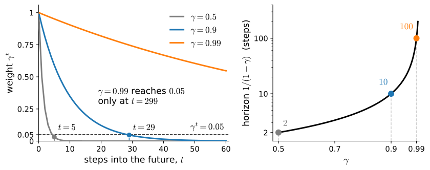
The first bound makes the objective finite; the second makes \(1/(1-\gamma)\) the effective horizon: the window within which rewards still carry appreciable weight. A scale, not a cliff: the fraction of a constant reward stream’s discounted mass lying past step \(k\) is exactly \(\gamma^k\), so 95 percent of the mass sits in the first \(\log 0.05 / \log \gamma\) steps, about three effective horizons (the third column of the table below). Read this way, \(\gamma = 0.99\) is not a magic number but a horizon of one hundred steps, and \(\gamma = 0.5\) is an agent that can barely see two steps ahead, myopic where \(\gamma\) near one is far-sighted. In numbers:
print(f'{"gamma":>6} {"horizon 1/(1-gamma)":>20} {"t: gamma^t < 0.05":>18}')
for g in [0.5, 0.9, 0.95, 0.99]:
    t5 = int(np.ceil(np.log(0.05) / np.log(g)))
    print(f'{g:>6} {1 / (1 - g):>20.0f} {t5:>18}')
gamma horizon 1/(1-gamma) t: gamma^t < 0.05
0.5 2 5
0.9 10 29
0.95 20 59
0.99 100 299print(f'{"gamma":>6} {"horizon 1/(1-gamma)":>20} {"t: gamma^t < 0.05":>18}')
for g in [0.5, 0.9, 0.95, 0.99]:
t5 = int(np.ceil(np.log(0.05) / np.log(g)))
print(f'{g:>6} {1 / (1 - g):>20.0f} {t5:>18}') gamma horizon 1/(1-gamma) t: gamma^t < 0.05
0.5 2 5
0.9 10 29
0.95 20 59
0.99 100 299Figure 14.1.2 plots the same facts. Our shortest path takes six moves, so the weight \(\gamma^5\) on the final reward must be worth acting for: about three percent at \(\gamma = 0.5\), a comfortable \(0.77\) at our \(\gamma = 0.95\). Choosing the discount is choosing how far the problem reaches into the future; it sits on the same design surface as the reward.
14.1.2.2 Episodes, Termination and Truncation
The trajectory we sampled ended in a hole. A state that ends the process is terminal; for analysis it can be represented as absorbing, every action leading back to it with reward zero. FrozenLake’s transition table happens to store the holes and the goal exactly that way, but the running episode simply ends and must be reset, so the absorbing continuation is a mathematical completion, not a simulator behavior to rely on. A run from start to a terminal state is an episode; tasks whose trajectories always end are episodic, unlike continuing tasks, where only the discount keeps the objective finite. The number of steps an episode may last is its horizon, and when episodes are bounded by \(T\) steps, a sum of \(T\) bounded rewards is finite already and \(\gamma = 1\) is legitimate.
Gymnasium’s step returns two flags whose difference is a fact about the MDP, not a software detail. terminated=True means the process entered a terminal state: the future is empty, worth exactly zero. truncated=True means we merely stopped watching, usually a time limit (FrozenLake cuts episodes at one hundred steps): the state has a future that our recording does not show. Merging the flags is fine for loop control, as in the cell above, and disastrous for value estimation, where treating a truncated state as worthless trains on a lie. The learning algorithms from Section 14.4 onward therefore mask bootstrapped targets with terminated alone; the exact computations of this section never needed a mask, because absorbing states at reward zero silence their own values.
14.1.3 The Choice of State
The kernel \(P(s' \mid s, a)\) conditions on the current state and action only: the Markov assumption, the “one assumption” of this section’s opening. Given the present, the past is irrelevant for predicting the future; whether that holds depends on what you call the state, and the choice is yours.
14.1.3.1 The Markov Assumption and State Augmentation
Let us think of a new agent where the state \(s_t\) is the location as above but the action \(a_t\) is the acceleration that the agent applies to its wheels instead of an abstract command like “go forward”. If this agent has some non-zero velocity at state \(s_t\), then the next location \(s_{t+1}\) is a function of the past location \(s_t\), the acceleration \(a_t\), and also the velocity of the agent at time \(t\), which is proportional to \(s_t - s_{t-1}\). This indicates that we should have
\[s_{t+1} = \textrm{some function}(s_t, a_t, s_{t-1}); \tag{14.1.6}\]
the “some function” in our case would be Newton’s law of motion. This is quite different from our transition function that simply depends upon \(s_t\) and \(a_t\).
Markov systems are all systems where the next state \(s_{t+1}\) is only a function of the current state \(s_t\) and the action \(a_t\) taken at the current state. In Markov systems, the next state does not depend on which actions were taken in the past or the states that the agent was at in the past. For example, the new agent that has acceleration as the action above is not Markovian because the next location \(s_{t+1}\) depends upon the previous state \(s_{t-1}\) through the velocity. It may seem that the Markovian nature of a system is a restrictive assumption, but it is not so. Markov Decision Processes are still capable of modeling a very large class of real systems. For example, for our new agent, if we choose our state \(s_t\) to be the tuple \((\textrm{location}, \textrm{velocity})\) then the system is Markovian because its next state \((\textrm{location}_{t+1}, \textrm{velocity}_{t+1})\) depends only upon the current state \((\textrm{location}_t, \textrm{velocity}_t)\) and the action at the current state \(a_t\).
This move, state augmentation, is the standard repair: enlarge the state until the future depends only on it. The price is a larger state space, and what to pack into the state is one of the quiet design decisions of applied reinforcement learning. The repair also has a ceiling: the sufficient statistic may be unknown, too large to store, or simply not observable, and in the last case the principled replacement is a distribution over the hidden part, the belief of the next paragraph.
14.1.3.2 Partial Observability
Augmentation assumes you can observe what you add, and often you cannot: a poker player does not see the opponents’ cards. An agent that receives an observation \(o_t\) revealing only part of the state lives in a partially observable MDP, where exact treatments must reason over beliefs about the hidden state and become dramatically harder. The workaday remedy is augmentation applied to observations: feed the agent a short window of recent observations and call the window the state. The classic instance is Atari, where a single frame shows where the ball is but not where it is going, and stacking four frames restores enough of the Markov property to play well; exercise 1 makes precise what the frame is missing. These two chapters assume the observation is the state; this paragraph is the fence around that assumption.
14.1.4 Bandits, Degenerate MDPs and the Model-Based Axis
Two degenerate corners of the MDP, and one axis, organize much of what follows.
14.1.4.1 The Bandit as a One-State MDP
Delete the states. With \(|\mathcal{S}| = 1\), every episode is a single action followed by a reward draw: the multi-armed bandit, exploration in its purest form. Nothing remains to plan (no next state exists) or to discount; the problem is to learn which action pays best from noisy samples, while the samples cost whatever the inferior arms lose. When Section 14.4 needs to isolate exploration from everything else that makes reinforcement learning hard, the bandit is the instrument we reach for.
14.1.4.2 The Degenerate MDP: Deterministic Transitions, Terminal Reward
Keep the states but delete the randomness and the intermediate payments: transitions deterministic, reward zero everywhere except at termination. Our lake is halfway there already, since the consistency check showed its reward is terminal-only; make the ice non-slippery and the degeneracy is complete. It looks too simple to need this chapter’s machinery, yet it is exactly text generation viewed as a decision process: appending a token to a context is a deterministic transition, and a verifier or reward model pays once, at the end. When Section 15.7 builds that correspondence, the degeneracies will remove terms from our algorithms rather than add any.
14.1.4.3 Model-Based versus Model-Free Methods
Everything in this section used the model itself: we read \(P\) and \(r\) from the simulator, and every number was an exact expectation. Algorithms that plan with a known or learned model are model-based; Section 14.2 is the canonical example. Algorithms that only touch sampled transitions \((s, a, r, s')\) are model-free; they begin in Section 14.4 and dominate everything after, because nobody hands you env.unwrapped.P for an environment of interest. The axis matters for data too: a model can be queried anywhere, while samples arrive only where the agent goes.
With the model in hand, we can settle the debt this section owes. Because the true reward pays only for finishing, learning will be slow, so consider a fix any practitioner might write: a bonus of \(0.3\) for every step that moves the agent closer to the goal, in expectation \(\tilde r(s, a) = r(s, a) + 0.3 \sum_{s'} P(s' \mid s, a) \, \mathbf{1}(d(s') < d(s))\) with \(d\) the Manhattan distance. It is not potential-based: approach is paid, retreat is not charged. We compute the policy it makes optimal by sweeping backup to convergence (the procedure gets its name in Section 14.2) and score both policies under the true reward by solving “my value is my reward plus the discounted value of where the kernel sends me”:
dist = abs(np.arange(16) // 4 - 3) + abs(np.arange(16) % 4 - 3)
closer = dist < dist[:, None, None]    # closer[s, :, s'] = 1 iff d(s') < d(s)
shaped = TabularMDP(mdp.P, mdp.r + 0.3 * (mdp.P * closer).sum(-1), gamma)

def greedy_sweeps(m):                  # repeated backups; named in next section
    V = np.zeros(m.num_states)
    for _ in range(500):
        V = m.backup(V).max(axis=1)
    return m.backup(V).argmax(axis=1), V

def exact_value(pi, s=0):              # V(s) under the true reward, exactly
    i = np.arange(mdp.num_states)
    return np.linalg.solve(np.eye(16) - gamma * mdp.P[i, pi], mdp.r[i, pi])[s]

pi_shaped, V_shaped = greedy_sweeps(shaped)
pi_true, V_true = greedy_sweeps(mdp)
print(f'shaped-optimal: at s=14 goes {"<v>^"[pi_shaped[14]]}, shaped value '
      f'{V_shaped[0]:.2f}, true value {exact_value(pi_shaped):.3f}')
print(f'true-optimal:   at s=14 goes {"<v>^"[pi_true[14]]}, true value '
      f'{exact_value(pi_true):.3f}')
shaped-optimal: at s=14 goes <, shaped value 2.15, true value 0.000
true-optimal: at s=14 goes v, true value 0.180dist = abs(np.arange(16) // 4 - 3) + abs(np.arange(16) % 4 - 3)
closer = dist < dist[:, None, None] # closer[s, :, s'] = 1 iff d(s') < d(s)
shaped = TabularMDP(mdp.P, mdp.r + 0.3 * (mdp.P * closer).sum(-1), gamma)
def greedy_sweeps(m): # repeated backups; named in next section
V = np.zeros(m.num_states)
for _ in range(500):
V = m.backup(V).max(axis=1)
return m.backup(V).argmax(axis=1), V
def exact_value(pi, s=0): # V(s) under the true reward, exactly
i = np.arange(mdp.num_states)
return np.linalg.solve(np.eye(16) - gamma * mdp.P[i, pi], mdp.r[i, pi])[s]
pi_shaped, V_shaped = greedy_sweeps(shaped)
pi_true, V_true = greedy_sweeps(mdp)
print(f'shaped-optimal: at s=14 goes {"<v>^"[pi_shaped[14]]}, shaped value '
f'{V_shaped[0]:.2f}, true value {exact_value(pi_shaped):.3f}')
print(f'true-optimal: at s=14 goes {"<v>^"[pi_true[14]]}, true value '
f'{exact_value(pi_true):.3f}')shaped-optimal: at s=14 goes <, shaped value 2.15, true value 0.000
true-optimal: at s=14 goes v, true value 0.180Look at state 14, the only cell from which the goal can be entered. The true optimum commands down there, and a third of those outcomes finish the task. The shaped optimum commands left, whose three outcomes are 10, 13 and 14: none is the goal, and no other cell borders the goal, so this policy can never finish. Its true value is exactly zero, while by the yardstick we wrote it is a star, worth \(2.15\) against the true optimum’s \(0.180\). The optimizer has discovered that a task that ends is a bonus stream that stops. Nobody wanted this policy; the reward asked for it. The failure is quiet: at a bonus of \(0.1\) (rerun the cell) the shaped optimum still reaches the goal, so nothing announces the cliff. Exercise 4 repairs the bonus with a potential.
14.1.5 Summary
A Markov decision process is four objects, \((\mathcal{S}, \mathcal{A}, P, r)\): states, actions, a transition kernel giving the distribution of the next state, and a reward defining the task. Its one assumption is that the state carries everything the past could say about the future, and that is a property of your modeling, not of the world: augment the state until it holds, where you can observe and afford what the augmentation needs; where you cannot, the problem is partially observed. The objective is the expected discounted return, and the discount is an effective horizon \(1/(1-\gamma)\): rewards beyond roughly that many steps are geometrically negligible, so \(\gamma = 0.99\) means “care about the next hundred steps”. Terminal states end the future; truncation ends only the recording, and confusing the two corrupts value estimates. The one-state MDP is the bandit, the deterministic terminal-reward MDP is text generation in disguise, and the first question to ask of any algorithm is whether it uses the kernel or only samples from it. Above all, the reward is authored, an optimizer is an adversary of sloppy authorship, and only potential-based reshaping with a potential that vanishes at episode-ending states is guaranteed harmless.
What the experiments show, and what they do not. Every number in this section is an exact computation on a known sixteen-state model: no learning, no seeds to vary, and any rerun reproduces it to the digit, except the single sampled trajectory, one draw shown for concreteness. The reward-hacking demonstration is an existence proof on one map with one bonus size: it shows the attack surface is real, not that every shaped reward fails, and at smaller bonuses the exploit disappears while the policy is still subtly distorted. It shows none of the difficulties of learning (estimation from samples, exploration, function approximation), which the rest of these two chapters measures.
14.1.6 Exercises
- [conceptual] What the state must contain. A single frame of Pong shows where the ball is but not where it is going, so the frame alone is not a state in the sense of Section 14.1. Say precisely which property of Equation 14.1.1 fails, give the smallest augmentation of the frame that restores it, and explain why the standard practice of stacking four frames is more than the minimum. Then do the same for MountainCar: name its state and action sets, and say what the environment would have to report instead for the position alone to be Markov.
- [short-code] Look at a transition function. Build the slippery FrozenLake MDP with
mdp = d2l.TabularMDP.from_gym(gym.make('FrozenLake-v1', is_slippery=True), gamma). Verify that every row ofmdp.Psums to one, and count how many state-action pairs have more than one possible successor. Repeat withis_slippery=False. How many numbers does the deterministic MDP need, and how many does the slippery one need? - [short-code] The effective horizon. Rewards in this book are bounded by some \(r_{\max}\). Show that the tail of the discounted return past step \(k\) is at most \(\gamma^k r_{\max} / (1 - \gamma)\), and find, for \(\gamma \in \{0.9, 0.95, 0.99, 0.999\}\), the smallest \(k\) at which that tail is below one percent of the maximum possible return. Plot \(k\) against \(1/(1-\gamma)\). Our gridworld’s optimal path is six steps long: which of these discount factors can even see the goal?
- [conceptual] Reward design and its failure. The gridworld pays \(1\) at the goal and nothing elsewhere, which makes learning slow. The section’s shaped reward paid the agent for getting closer to the goal, and the policy it made optimal never reached the goal at all. Consider the closely related two-sided form \(r(s, a) = d(s) - d(s')\) with \(d\) the Manhattan distance. Show that on a map with a wall this too can make a policy that never reaches the goal earn more than one that does. Then show that the potential-based form \(r(s,a) + \gamma \Phi(s') - \Phi(s)\) leaves the optimal policy unchanged for any function \(\Phi\) with \(\Phi = 0\) at terminal states: write out the telescoping sum for an episode of length \(T\), exhibit the residual \(\gamma^T \Phi(s_T)\) that survives at the endpoint, and give the two ways to kill it (the zero boundary condition, or continuing the shaped reward through the absorbing state). Finally, identify what goes wrong with the naive fixes in that language.
- [conceptual] Random rewards. Section 14.1 notes that a random reward can be folded into \(r(s,a)\) by taking its mean. Make this precise: let the reward at \((s,a)\) be a random variable \(R\) with \(E[R] = r(s,a)\), drawn independently at each visit. Show that the value function of every policy is unchanged. Where, then, does the randomness of \(R\) show up at all?
- [conceptual] Which problems are not MDPs. For each of the following, say whether it is an MDP under the obvious choice of state, and if not, what to add: a poker hand; a robot whose battery drains; a recommender that a user grows tired of; a chess position with the fifty-move rule.