%matplotlib inline
from d2l import torch as d2l
import gymnasium as gym
import numpy as np
import torch
from torch import nn14.3 Learning from Demonstrations
Dynamic programming consumed the whole model: every number in Section 14.2 was computed from the kernel \(P\) and the reward \(r\). This section throws both away and replaces them with something far more common in practice: someone who can already do the task. Given demonstrations from an expert, copying them is supervised learning, a classification problem we solved in Section 3.1, and it costs no reinforcement learning at all. So this section asks strictly less than the last one, and for thirty lines of code the free lunch is real: the cloned policy is flawless on its training data. Then we measure it acting on its own, watch it lose most of the expert’s return, prove that the loss scales with the square of the horizon, and fix it by changing nothing about the model and everything about where the data comes from. That failure and its repair are the sharpest argument for the rest of these two chapters: an agent’s mistakes are priced not per decision but per trajectory, because the agent must live in the states its own decisions create.
%matplotlib inline
from d2l import jax as d2l
from flax import nnx
import gymnasium as gym
import jax
from jax import numpy as jnp
import numpy as np
import optax
14.3.1 Behavior Cloning
A demonstration is a recorded trajectory of an expert doing the task. Demonstration data in the wild may carry more: next states, timing, goals, sometimes rewards. Behavior cloning, this section’s method, consumes exactly two columns of it, the states visited and the actions taken, so two columns are all our recorder keeps. No reward is logged, and no transition kernel is consulted; whoever demonstrates does not know a kernel exists. Experts are cheap to find in exactly the situations where models are not: a driver steering a vehicle, a surgeon suturing, a human writing a helpful answer. On the slippery lake we are luckier still, because Section 14.2 can manufacture the expert: we compute \(\pi^*\) by value iteration one last time, let it demonstrate, and then lock the machinery away. The learner will see only what a learner ever sees, pairs \((s, a)\); keeping the solved lake underneath means every claim in this section can be checked against ground truth.
14.3.1.1 The Reduction to Classification
Imitation is the oldest shortcut in the field: in 1989 the ALVINN system already drove a van by training a small network to map camera images to a demonstrated driver’s steering commands (Pomerleau 1991). Our expert demonstrates three episodes:
gamma = 0.95
env = gym.make('FrozenLake-v1', is_slippery=True)
mdp = d2l.TabularMDP.from_gym(env, gamma)
V_star = d2l.value_iteration(mdp, num_iters=1000)[-1]
pi_star = mdp.backup(V_star).argmax(axis=1)

def demonstrations(num_episodes):
    """Roll the expert; record only what it saw and what it did."""
    states, actions = [], []
    for _ in range(num_episodes):
        s, done = env.reset()[0], False
        while not done:
            states.append(s)
            actions.append(int(pi_star[s]))
            s, reward, terminated, truncated, _ = env.step(actions[-1])
            done = terminated or truncated
    return np.array(states), np.array(actions)

env.reset(seed=0)
demo_s, demo_a = demonstrations(3)
print(f'{demo_s.size} state-action pairs from 3 expert episodes, '
      f'covering {np.unique(demo_s).size} of 11 reachable states')
96 state-action pairs from 3 expert episodes, covering 7 of 11 reachable statesgamma = 0.95
env = gym.make('FrozenLake-v1', is_slippery=True)
mdp = d2l.TabularMDP.from_gym(env, gamma)
V_star = d2l.value_iteration(mdp, num_iters=1000)[-1]
pi_star = mdp.backup(V_star).argmax(axis=1)
def demonstrations(num_episodes):
"""Roll the expert; record only what it saw and what it did."""
states, actions = [], []
for _ in range(num_episodes):
s, done = env.reset()[0], False
while not done:
states.append(s)
actions.append(int(pi_star[s]))
s, reward, terminated, truncated, _ = env.step(actions[-1])
done = terminated or truncated
return np.array(states), np.array(actions)
env.reset(seed=0)
demo_s, demo_a = demonstrations(3)
print(f'{demo_s.size} state-action pairs from 3 expert episodes, '
f'covering {np.unique(demo_s).size} of 11 reachable states')96 state-action pairs from 3 expert episodes, covering 7 of 11 reachable statesThree episodes on slippery ice wander long enough to produce 96 labeled pairs, but they happen to visit only 7 of the 11 frozen cells: the three top-row states and, fatefully, state 13 never appear. Keep that in mind; the fit cannot know what it was never shown.
Behavior cloning treats these pairs exactly as Section 3.1 treated images and labels: the state is the input, the expert’s action is the class, and we fit a conditional distribution \(\pi_\theta(a \mid s)\) by maximizing the log-likelihood \(\sum_i \log \pi_\theta(a_i \mid s_i)\), that is, by minimizing cross-entropy. All it needs is a parameterized policy, and the object we now build is the one that will carry every learned policy for the rest of these two chapters:
class ActorCritic(nn.Module):
    """A policy and a value function, each with its own optimizer."""
    def __init__(self, policy, value, lr=1e-2):
        super().__init__()
        self.policy, self.value = policy, value
        self.opt_pi = torch.optim.Adam(policy.parameters(), lr=lr)
        self.opt_v = torch.optim.Adam(value.parameters(), lr=lr)

    def forward(self, obs):
        return torch.softmax(self.policy(obs), dim=-1)

    def log_prob(self, obs, act):
        """log pi(a|s) for a batch of states and the actions taken there."""
        return torch.log_softmax(self.policy(obs), dim=-1) \
                    .gather(-1, act[:, None]).squeeze(-1)

    def V(self, obs):
        return self.value(obs).squeeze(-1)

    @classmethod
    def tabular(cls, num_states, num_actions, lr=0.1):
        """One preference theta_{s,a} per state-action pair: an embedding."""
        policy, value = (nn.Embedding(num_states, num_actions),
                         nn.Embedding(num_states, 1))
        nn.init.zeros_(policy.weight), nn.init.zeros_(value.weight)
        return cls(policy, value, lr)
class ActorCritic(nnx.Module):
"""A policy and a value function, each with its own optimizer."""
def __init__(self, policy, value, lr=1e-2):
self.policy, self.value = policy, value
self.opt_pi = nnx.Optimizer(policy, optax.adam(lr), wrt=nnx.Param)
self.opt_v = nnx.Optimizer(value, optax.adam(lr), wrt=nnx.Param)
def log_prob(self, obs, act, policy=None):
"""log pi(a|s). Gradients flow w.r.t. the module you differentiate;
the update functions pass that module back in as `policy`."""
policy = self.policy if policy is None else policy
logp = jax.nn.log_softmax(policy(obs), axis=-1)
return jnp.take_along_axis(logp, act[:, None], axis=-1).squeeze(-1)
def V(self, obs, value=None):
value = self.value if value is None else value
return value(obs).squeeze(-1)
@classmethod
def tabular(cls, num_states, num_actions, lr=0.1, rngs=None):
"""One preference theta_{s,a} per state-action pair: an embedding."""
rngs = nnx.Rngs(d2l.get_key()) if rngs is None else rngs
zeros = nnx.initializers.zeros_init()
return cls(nnx.Embed(num_states, num_actions,
embedding_init=zeros, rngs=rngs),
nnx.Embed(num_states, 1, embedding_init=zeros, rngs=rngs),
lr)The tabular constructor is a softmax-regression model in a thin disguise: an embedding table holds one preference \(\theta_{s, a}\) per state-action pair, an integer state indexes its row, and a softmax turns the row into \(\pi_\theta(\cdot \mid s)\). Zero initialization makes the starting policy exactly uniform. The class also carries a value head and a second optimizer that nothing in this section touches: the container is named for the actor-critic architecture it will grow into, and introducing it here as a supervised-learning object is deliberate, because Section 14.5 will then need no new policy class, only a new way to choose the weights: no expert, only reward.
The environment, d2l.evaluate, and everything else we share between frameworks speaks numpy, so the class gets a numpy boundary: four small methods through which framework arrays leave the model. The torch tab must wrap them in no_grad; the JAX tab needs no equivalent, since nothing records a gradient graph outside an explicit grad trace:
@d2l.add_to_class(ActorCritic)
def act(self, obs, rng):
    """Sample an action; numpy in, int out, the acting protocol of evaluate."""
    with torch.no_grad():
        probs = torch.softmax(self.policy(torch.as_tensor(obs)), -1).numpy()
    return int(rng.choice(len(probs), p=probs))

@d2l.add_to_class(ActorCritic)
def act_greedy(self, obs, rng=None):
    with torch.no_grad():
        return int(self.policy(torch.as_tensor(obs)).argmax())

@d2l.add_to_class(ActorCritic)
def value_np(self, obs):
    with torch.no_grad():
        return self.V(torch.as_tensor(obs)).numpy()

@d2l.add_to_class(ActorCritic)
def log_prob_np(self, obs, act):
    with torch.no_grad():
        return self.log_prob(torch.as_tensor(obs),
torch.as_tensor(act)).numpy()@d2l.add_to_class(ActorCritic)
def act(self, obs, rng):
"""Sample an action; numpy in, int out, the acting protocol of evaluate."""
probs = np.asarray(jax.nn.softmax(self.policy(jnp.asarray(obs)), axis=-1))
return int(rng.choice(len(probs), p=probs))
@d2l.add_to_class(ActorCritic)
def act_greedy(self, obs, rng=None):
return int(self.policy(jnp.asarray(obs)).argmax())
@d2l.add_to_class(ActorCritic)
def value_np(self, obs):
return np.asarray(self.V(jnp.asarray(obs)))
@d2l.add_to_class(ActorCritic)
def log_prob_np(self, obs, act):
return np.asarray(self.log_prob(jnp.asarray(obs), jnp.asarray(act)))Both act methods draw from the shared numpy generator that gets passed in, never from a framework sampler, so all randomness an environment ever sees runs through one auditable stream. Only act_greedy and log_prob_np work today; sampling and the value reader earn their keep from Section 14.5 on. Now the fit, which is the six lines of Section 3.1 with the images replaced by states:
def clone(states, actions, num_steps=200):
    """Behavior cloning: cross-entropy fit of pi(a|s) to expert choices."""
    ac = ActorCritic.tabular(16, 4)
    obs, act = torch.as_tensor(states), torch.as_tensor(actions)
    for _ in range(num_steps):
        loss = -ac.log_prob(obs, act).mean()
        ac.opt_pi.zero_grad()
        loss.backward()
        ac.opt_pi.step()
    return ac, loss.item()

bc, nll = clone(demo_s, demo_a)
print(f'cross-entropy on the demonstrations after the fit: {nll:.3f}')
for s in (9, 3):
    probs = np.exp(bc.log_prob_np(np.repeat(s, 4), np.arange(4)))
    print(f'clone pi(.|s={s}): {np.round(probs, 3)}')
cross-entropy on the demonstrations after the fit: 0.004
clone pi(.|s=9): [0.001 0.996 0.001 0.001]
clone pi(.|s=3): [0.25 0.25 0.25 0.25]def clone(states, actions, num_steps=200):
"""Behavior cloning: cross-entropy fit of pi(a|s) to expert choices."""
ac = ActorCritic.tabular(16, 4)
obs, act = jnp.asarray(states), jnp.asarray(actions)
def nll_fn(policy):
return -ac.log_prob(obs, act, policy).mean()
for _ in range(num_steps):
loss, grads = nnx.value_and_grad(nll_fn)(ac.policy)
ac.opt_pi.update(ac.policy, grads)
return ac, float(loss)
bc, nll = clone(demo_s, demo_a)
print(f'cross-entropy on the demonstrations after the fit: {nll:.3f}')
for s in (9, 3):
probs = np.exp(bc.log_prob_np(np.repeat(s, 4), np.arange(4)))
print(f'clone pi(.|s={s}): {np.round(probs, 3)}')cross-entropy on the demonstrations after the fit: 0.004
clone pi(.|s=9): [0.001 0.996 0.001 0.001]
clone pi(.|s=3): [0.25 0.25 0.25 0.25]The loss is driven essentially to zero, and the two probed rows say why this problem is easy and what its limits are. At state 9, demonstrated many times with the same label, the clone is all but certain of down. At state 3, never demonstrated, the row of the table was never touched by a gradient: the policy is exactly uniform, because where there was no data, the fit has no opinion. Greedy action selection breaks that four-way tie by picking action 0, left, an arbitrary choice that no one made on purpose.
One last piece of packaging. The cloning update is one ascent step on a weighted sum of log-probabilities with all weights equal to one, and it is worth saving under the name every later section will call it by. Its batch argument is any object carrying obs and act arrays; the container that plays this role from Section 14.5 onward is built there, and from then on the weights carry information about returns rather than a teacher’s endorsement:
def policy_step(ac, batch, advantage):
    """One ascent step on E[A_t log pi(a_t|s_t)]; A_t arrives as numpy = data."""
    obs, act = torch.as_tensor(batch.obs), torch.as_tensor(batch.act)
    adv = torch.as_tensor(advantage)
    loss = -(adv * ac.log_prob(obs, act)).mean()
    ac.opt_pi.zero_grad()
    loss.backward()
    ac.opt_pi.step()
    return loss.item()
def policy_step(ac, batch, advantage):
"""One ascent step on E[A_t log pi(a_t|s_t)]; A_t arrives as numpy = data.
Not jitted: batches change shape at every update; jit would recompile."""
obs, act = jnp.asarray(batch.obs), jnp.asarray(batch.act)
adv = jnp.asarray(advantage)
loss, grads = nnx.value_and_grad(
lambda policy: -(adv * ac.log_prob(obs, act, policy)).mean())(ac.policy)
ac.opt_pi.update(ac.policy, grads)
return float(loss)Note what the signature enforces: the weights arrive as a numpy array, and a numpy array cannot carry a gradient graph, so the weighting is data by construction, in both frameworks, with no detach and no stop-gradient in sight.
14.3.1.2 The Train-Equals-Test Assumption
A classifier’s guarantee has fine print: it promises accuracy on the distribution it was trained on. That is the train-equals-test assumption of Section 3.7, and behavior cloning inherits it in a treacherous form, because the clone is not tested on the expert’s states. It is tested on the states that its own actions produce. The moment it deviates once, it is its own distribution’s author. We measure both sides of the fine print, using the evaluate protocol of Section 14.2, in which a policy is any function from observation to action, so the method bc.act_greedy can be passed as it is:
env.reset(seed=1)
expert_rate = d2l.evaluate(env, lambda s, rng: int(pi_star[s]),
                           num_episodes=1000)
clone_rate = d2l.evaluate(env, bc.act_greedy, num_episodes=1000)
mistakes = sum(bc.act_greedy(s) != a for s, a in zip(demo_s, demo_a))
print(f'mistakes on the {demo_s.size} demonstration pairs: {mistakes}')
print(f'success rate: expert {expert_rate:.1%}, clone {clone_rate:.1%}')
mistakes on the 96 demonstration pairs: 0
success rate: expert 73.4%, clone 17.5%env.reset(seed=1)
expert_rate = d2l.evaluate(env, lambda s, rng: int(pi_star[s]),
num_episodes=1000)
clone_rate = d2l.evaluate(env, bc.act_greedy, num_episodes=1000)
mistakes = sum(bc.act_greedy(s) != a for s, a in zip(demo_s, demo_a))
print(f'mistakes on the {demo_s.size} demonstration pairs: {mistakes}')
print(f'success rate: expert {expert_rate:.1%}, clone {clone_rate:.1%}')mistakes on the 96 demonstration pairs: 0
success rate: expert 73.4%, clone 17.5%Zero mistakes, and a quarter of the expert’s success rate. As a classifier the clone is perfect; as an agent it fails three times as often as an expert who reaches the goal three times out of four. The mechanism is the ice: slips push the clone into the states its dataset never covered, and one of them, state 13, is catastrophic to get wrong, since it borders the hole at 12, the expert escapes it by commanding right, and the clone’s arbitrary left points the intended move straight into the hole. How typical was our unlucky dataset? We redraw it ten times at three sizes, refitting each time (only briefly, since the argmax of each row settles long before the digits of the loss do, the same policies-before-values effect as in Section 14.2):
env.reset(seed=2)
for n in [1, 3, 10]:
    rates = []
    for _ in range(10):
        ac, _ = clone(*demonstrations(n), num_steps=50)
        tab = np.array([ac.act_greedy(s) for s in range(16)])
        rates.append(d2l.evaluate(env, lambda s, rng: int(tab[s]),
                                  num_episodes=300))
    rates = np.sort(np.array(rates))
    print(f'{n:>2} episodes: median success {np.median(rates):.0%}, '
          f'worst {rates[0]:.0%}, over ten datasets')
1 episodes: median success 44%, worst 0%, over ten datasets
3 episodes: median success 73%, worst 70%, over ten datasets
10 episodes: median success 73%, worst 70%, over ten datasetsenv.reset(seed=2)
for n in [1, 3, 10]:
rates = []
for _ in range(10):
ac, _ = clone(*demonstrations(n), num_steps=50)
tab = np.array([ac.act_greedy(s) for s in range(16)])
rates.append(d2l.evaluate(env, lambda s, rng: int(tab[s]),
num_episodes=300))
rates = np.sort(np.array(rates))
print(f'{n:>2} episodes: median success {np.median(rates):.0%}, '
f'worst {rates[0]:.0%}, over ten datasets') 1 episodes: median success 44%, worst 0%, over ten datasets
3 episodes: median success 73%, worst 70%, over ten datasets
10 episodes: median success 73%, worst 70%, over ten datasetsThe median dataset clones this small lake well even at three episodes; the tail is the story. A single-episode dataset can produce a clone that never reaches the goal, and the disaster our own three-episode draw produced is no anomaly, just a draw from that tail. More demonstrations make bad draws rarer, but notice what they do not shrink: the size of the loss when a gap in coverage does bite. That is set by the horizon, not by the dataset, and it is time to say so precisely.
14.3.2 Compounding Error
14.3.2.1 The Error Bounds: \(\varepsilon T^2\) versus \(\varepsilon T\)
Supervised learning controls the probability of error per decision. Acting composes decisions, and the composition is where the quadratic comes from. Write \(d^\pi_t\) for the distribution over states that an agent following \(\pi\) occupies at step \(t\); “the expert’s distribution” means the states weighted by \(d^{\pi^*}_t\), which is exactly what a demonstration dataset samples.
Proposition (compounding error). Consider an episodic task with horizon \(T\) and per-step rewards in \([0, 1]\). Let \(\hat\pi\) disagree with the expert with probability at most \(\varepsilon\) per step. (i) If the disagreement is measured under the expert’s state distribution, the expected return of \(\hat\pi\) can fall short of the expert’s by \(\Theta(\varepsilon T^2)\). (ii) If it is measured under \(\hat\pi\)’s own state distribution, and a single deviation followed by expert behavior costs at most \(u\) return, the shortfall is at most \(u\,\varepsilon T = O(\varepsilon T)\) (Ross et al. 2011).
Proof. Run \(\hat\pi\) and mark the first step at which it deviates from the expert. Until the mark, its states are distributed as the expert’s, so the guarantee applies there, and the mark falls at step \(t\) with probability at most \(\varepsilon\). From the mark on, \(\hat\pi\) occupies states that the expert’s distribution never weighted: \(\varepsilon\) was measured where the expert goes, not where \(\hat\pi\) ends up, so nothing bounds its behavior there, and in the worst case it forfeits every remaining reward, up to \(T - t\). Summing over when the mark falls, the shortfall is at most \(\sum_{t \leq T} \varepsilon\,(T - t) \leq \varepsilon T^2 / 2\), and the chain below achieves this rate, so it is tight. For (ii), walk along \(\hat\pi\)’s own trajectory and exchange its action for the expert’s one step at a time: the exchange at step \(t\) is needed with probability at most \(\varepsilon\), measured exactly where \(\hat\pi\) is, and repairing it costs at most \(u\); summing gives \(u \varepsilon T\). \(\blacksquare\)
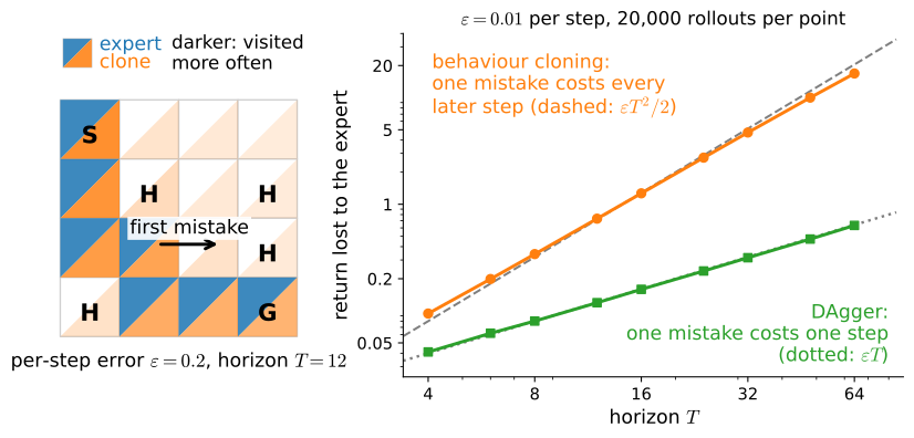
The one step that matters is the italicized one: the same \(\varepsilon\) buys a guarantee an order of \(T\) stronger when it holds on the learner’s own distribution. Figure 14.3.1 draws both halves, and we can measure them on an environment built to isolate the mechanism: a chain of ten states in which the expert steps right and collects one unit of reward per step, and an imitator disagrees with probability \(\varepsilon = 0.05\) at each step. For the cloned imitator a first disagreement is fatal (it has never seen an off-chain state), which is the worst case that step (2) of the proof allows; a recovering imitator gets back on the chain one step later, losing exactly the step it fumbled, which is case (ii) with \(u = 1\):
eps, T_max = 0.05, 10
rng = np.random.default_rng(3)
wrong = rng.random((20000, T_max)) < eps
T = np.arange(1, T_max + 1)
gap_bc = T - np.cumprod(~wrong, axis=1).cumsum(axis=1).mean(axis=0)
gap_rec = T - (~wrong).cumsum(axis=1).mean(axis=0)
d2l.plot([T] * 4, [gap_bc, eps * T ** 2 / 2, gap_rec, eps * T],
         xlabel='horizon T', ylabel='return lost to the expert',
         legend=['cloned', '$\\varepsilon T^2/2$', 'recovering',
                 '$\\varepsilon T$'],
         xscale='log', yscale='log', figsize=(5, 3.5))
print(f'lost return at T={T_max}: cloned {gap_bc[-1]:.2f} '
      f'(eps T^2/2 = {eps * T_max ** 2 / 2:.2f}), '
      f'recovering {gap_rec[-1]:.2f} (eps T = {eps * T_max:.2f})')
lost return at T=10: cloned 2.40 (eps T^2/2 = 2.50), recovering 0.51 (eps T = 0.50)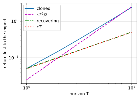
eps, T_max = 0.05, 10
rng = np.random.default_rng(3)
wrong = rng.random((20000, T_max)) < eps
T = np.arange(1, T_max + 1)
gap_bc = T - np.cumprod(~wrong, axis=1).cumsum(axis=1).mean(axis=0)
gap_rec = T - (~wrong).cumsum(axis=1).mean(axis=0)
d2l.plot([T] * 4, [gap_bc, eps * T ** 2 / 2, gap_rec, eps * T],
         xlabel='horizon T', ylabel='return lost to the expert',
         legend=['cloned', '$\\varepsilon T^2/2$', 'recovering',
                 '$\\varepsilon T$'],
         xscale='log', yscale='log', figsize=(5, 3.5))
print(f'lost return at T={T_max}: cloned {gap_bc[-1]:.2f} '
      f'(eps T^2/2 = {eps * T_max ** 2 / 2:.2f}), '
      f'recovering {gap_rec[-1]:.2f} (eps T = {eps * T_max:.2f})')
lost return at T=10: cloned 2.40 (eps T^2/2 = 2.50), recovering 0.51 (eps T = 0.50)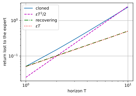
On logarithmic axes the two measurements are straight lines of different slopes: the cloned imitator tracks the quadratic reference and the recovering one the linear reference, already five times apart at \(T = 10\). Panel (b) of Figure 14.3.1 runs the same simulation at \(\varepsilon = 0.01\) out to \(T = 64\), where the gap between the rates has grown past thirtyfold.
14.3.2.2 The Divergence of the State Distributions
It is tempting to blame the optimizer, or the model class, or the small dataset, and all three are innocent: the classifier met its specification exactly, with zero training mistakes. What broke is the specification’s premise. The distribution the clone faces at test time is not the one it was certified on, and the divergence between the two is not noise but a computable object. On the lake we can evolve both state distributions exactly, one step of the kernel at a time, expert dynamics against clone dynamics from the same start state:
pi_clone = np.array([bc.act_greedy(s) for s in range(16)])
states = np.arange(16)
P_exp, P_clo = mdp.P[states, pi_star], mdp.P[states, pi_clone]
d_exp = d_clo = np.eye(16)[0]
occ_exp, occ_clo = np.zeros(16), np.zeros(16)
for t in range(1, 21):
    d_exp, d_clo = d_exp @ P_exp, d_clo @ P_clo
    occ_exp, occ_clo = occ_exp + d_exp, occ_clo + d_clo
    if t in (3, 5, 10, 20):
        print(f'after {t:>2} steps: total variation '
              f'{0.5 * np.abs(d_exp - d_clo).sum():.3f}')
print(f'mass in the hole at s=12 after 20 steps: '
      f'expert {d_exp[12]:.3f}, clone {d_clo[12]:.3f}')
d2l.show_grid(env.unwrapped.desc, np.stack([occ_exp, occ_clo]) / 20,
              np.stack([pi_star, pi_clone]),
              titles=['expert occupancy', 'clone occupancy'])
after 3 steps: total variation 0.000
after 5 steps: total variation 0.004
after 10 steps: total variation 0.063
after 20 steps: total variation 0.227
mass in the hole at s=12 after 20 steps: expert 0.000, clone 0.221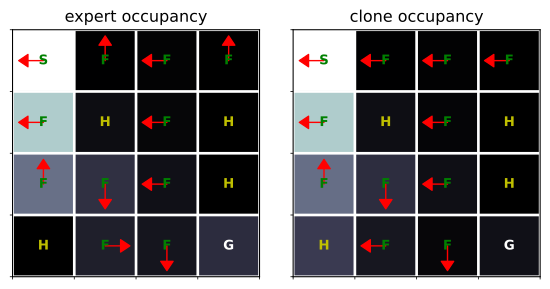
pi_clone = np.array([bc.act_greedy(s) for s in range(16)])
states = np.arange(16)
P_exp, P_clo = mdp.P[states, pi_star], mdp.P[states, pi_clone]
d_exp = d_clo = np.eye(16)[0]
occ_exp, occ_clo = np.zeros(16), np.zeros(16)
for t in range(1, 21):
    d_exp, d_clo = d_exp @ P_exp, d_clo @ P_clo
    occ_exp, occ_clo = occ_exp + d_exp, occ_clo + d_clo
    if t in (3, 5, 10, 20):
        print(f'after {t:>2} steps: total variation '
              f'{0.5 * np.abs(d_exp - d_clo).sum():.3f}')
print(f'mass in the hole at s=12 after 20 steps: '
      f'expert {d_exp[12]:.3f}, clone {d_clo[12]:.3f}')
d2l.show_grid(env.unwrapped.desc, np.stack([occ_exp, occ_clo]) / 20,
              np.stack([pi_star, pi_clone]),
              titles=['expert occupancy', 'clone occupancy'])
after 3 steps: total variation 0.000
after 5 steps: total variation 0.004
after 10 steps: total variation 0.063
after 20 steps: total variation 0.227
mass in the hole at s=12 after 20 steps: expert 0.000, clone 0.221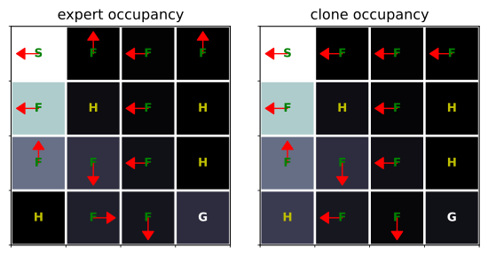
For the first three steps the two distributions are identical: the clone acts exactly like the expert until the ice has had time to push it somewhere it was never taught, which is the proof’s coupling argument printed as data. Then the gap opens and keeps growing, and by step 20 the clone has parked 22 percent of its probability mass in the hole at 12, beside state 13, a cell the expert enters with probability exactly zero. The two occupancy maps show the same story cell by cell: nearly identical mass where the demonstrations reached, and the clone’s surplus sitting in the one hole and on its doorstep, under the arrow that points into it. This is the chapter’s founding difficulty in its purest form. The agent generates its own data, so even a perfect teacher with a perfect student fails if the student is only certified on the teacher’s states; the certificate expires the moment the first mistake, or here the first slip, moves the test distribution.
14.3.3 Interactive Data Collection
14.3.3.1 DAgger: Dataset Aggregation
The proposition does not just diagnose; it prescribes. Both of its cases have the same \(\varepsilon\), and the linear one holds when the error is small on the learner’s own distribution, so the fix is to put the training data there: roll the learner, keep the states it actually visits, ask the expert after the fact what it would have done at each of them, and refit on everything collected so far. This is DAgger, dataset aggregation (Ross et al. 2011), and it is one relabeling step away from behavior cloning:
def relabel(ac, num_episodes):
    """Roll the learner; label its states with the expert's action."""
    visited = []
    for _ in range(num_episodes):
        s, done = env.reset()[0], False
        while not done:
            visited.append(s)
            s, reward, terminated, truncated, _ = env.step(ac.act_greedy(s))
            done = terminated or truncated
    visited = np.array(visited)
    return visited, pi_star[visited]

env.reset(seed=4)
agg_s, agg_a = demo_s, demo_a
for k in range(4):
    dag, _ = clone(agg_s, agg_a)
    tab = np.array([dag.act_greedy(s) for s in range(16)])
    rate = d2l.evaluate(env, lambda s, rng: int(tab[s]), num_episodes=1000)
    print(f'round {k}: trained on {agg_s.size:>3} pairs, '
          f'success rate {rate:.1%}')
    new_s, new_a = relabel(dag, 3)
    agg_s, agg_a = (np.concatenate([agg_s, new_s]),
                    np.concatenate([agg_a, new_a]))
round 0: trained on 96 pairs, success rate 18.0%
round 1: trained on 188 pairs, success rate 72.0%
round 2: trained on 273 pairs, success rate 72.2%
round 3: trained on 426 pairs, success rate 71.9%def relabel(ac, num_episodes):
"""Roll the learner; label its states with the expert's action."""
visited = []
for _ in range(num_episodes):
s, done = env.reset()[0], False
while not done:
visited.append(s)
s, reward, terminated, truncated, _ = env.step(ac.act_greedy(s))
done = terminated or truncated
visited = np.array(visited)
return visited, pi_star[visited]
env.reset(seed=4)
agg_s, agg_a = demo_s, demo_a
for k in range(4):
dag, _ = clone(agg_s, agg_a)
tab = np.array([dag.act_greedy(s) for s in range(16)])
rate = d2l.evaluate(env, lambda s, rng: int(tab[s]), num_episodes=1000)
print(f'round {k}: trained on {agg_s.size:>3} pairs, '
f'success rate {rate:.1%}')
new_s, new_a = relabel(dag, 3)
agg_s, agg_a = (np.concatenate([agg_s, new_s]),
np.concatenate([agg_a, new_a]))round 0: trained on 96 pairs, success rate 18.0%
round 1: trained on 188 pairs, success rate 72.0%
round 2: trained on 273 pairs, success rate 72.2%
round 3: trained on 426 pairs, success rate 71.9%Round 0 is behavior cloning on the original 96 pairs, back at its familiar failure. One round later the clone matches the expert. Nothing about the model, the loss, or the optimizer changed; only the sampling distribution did, and it repaired in three relabeled episodes what the ten-dataset sweep above suggested would take an order of magnitude more expert-only episodes to make reliable. The reason is precision, not volume: the learner’s own rollouts spend their time exactly where the learner goes wrong, state 13 above all, so the first batch of corrections lands on the very rows of the table that caused the failure. No sampling scheme built on the expert’s distribution can promise that, because the expert does not visit the learner’s mistakes. Keep the demonstration in scope, though: that one round suffices is a fact about this small lake, and what ran here is a miniature of distribution repair, not the algorithm the guarantee covers. DAgger’s theorem (Ross et al. 2011) is a reduction to online learning, and to bound the final policy’s cost it needs the full loop: iterated collection, a no-regret learner trained on the aggregated dataset, and in the original analysis a mixture of expert and learner during collection. The price is also on a different axis: DAgger needs the expert on call to label states after the fact, not just a recorded dataset, and exercise 4 accounts for the two methods at an equal query budget. Aggregating rather than replacing the data is load-bearing even in miniature: each round’s dataset contains all previous rounds, so the sequence of fits stabilizes rather than chasing its own latest mistakes.
14.3.3.2 Supervised Fine-Tuning and Offline RL
Twice in this book, once soon and once at scale. Supervised fine-tuning of a language model is behavior cloning, term for term: the state is the context, the action is the next token, the demonstrations are curated responses, and the fitted model is then deployed on contexts that it wrote itself. The proposition prices what happens next: a model tuned only on gold responses drifts off its training distribution as generations grow long, and the drift compounds; that is where Section 15.7 picks the story up. Closer by, behavior cloning is the standing baseline of offline reinforcement learning: given a fixed dataset of logged behavior and no interaction at all, cloning it is always available, and every method in Section 15.6 must justify itself against that baseline.
14.3.3.3 Modern Imitation Learning
Modern imitation learning mostly relaxes what the expert must provide. Generative adversarial imitation learning dispenses with action labels on the learner’s states: a discriminator learns to distinguish learner trajectories from expert ones, and its confusion is handed to a reinforcement-learning algorithm as a reward (Ho and Ermon 2016). Maximum-entropy inverse reinforcement learning inverts the problem, inferring the reward function under which the demonstrations are (softly) optimal and planning against it (Ziebart et al. 2008). And diffusion policies replace the softmax head with a diffusion model over action sequences, so that multimodal demonstrations (two equally good ways around an obstacle) are represented rather than averaged into something in between; they are the workhorse of current robot-manipulation imitation (Chi et al. 2023). All three inherit this section’s geometry: whatever plays the role of the fit, the distribution it is tested on is the learner’s own.
14.3.4 Summary
Behavior cloning reduces imitation to classification: fit \(\pi_\theta(a \mid s)\) to demonstrated pairs by cross-entropy, exactly the softmax regression of Section 3.1, requiring neither the kernel nor a reward. The reduction is real and so is its fine print: the classifier is certified on the expert’s state distribution, while the deployed policy is tested on its own, and the two diverge as soon as one mistake or one slip of the ice moves the agent off the demonstrated states. Quantitatively, a per-step error \(\varepsilon\) under the expert’s distribution can cost \(\Theta(\varepsilon T^2)\) return over horizon \(T\), while the same error under the learner’s own distribution costs \(O(\varepsilon T)\); the missing guarantee off-distribution is the whole difference. DAgger moves the training distribution to where the second case needs it, the learner’s own states, by collecting from the learner and relabeling with the expert, at the price of keeping the expert on call; its formal guarantee is for the iterated, no-regret version, and our one round demonstrated the mechanism rather than the theorem. The section also introduced the two objects that carry the rest of these chapters: the ActorCritic container, whose tabular policy is an embedding table behind a softmax, and policy_step, the weighted log-likelihood ascent step of which cloning is the all-weights-one special case.
What the experiments show, and what they do not. Every printed number is deterministic given the stated seeds, and the shared cells print identically in both frameworks; the two learned fits are deterministic too, zero-initialized and full-batch, so reruns reproduce them to the digit. The headline comparison (zero training mistakes, 73.4 percent against 17.5 percent success) is one deliberately unlucky three-episode draw whose typicality the ten-dataset sweep quantifies: most small datasets clone this lake to within a few points of the expert, and a persistent minority fail badly. The chain experiment realizes the proposition’s two extreme cases by construction, an imitator that never recovers and one that always does; real tasks live between the rates, not on them. And nothing here touches the harder problem these chapters exist for: what to do when there is no expert at all, which begins in Section 14.4, with samples replacing sums.
14.3.5 Exercises
- [conceptual] Where the bound comes from. Reproduce the \(O(\varepsilon T^2)\) argument and identify the one step where “the expert’s distribution” is replaced by “the learner’s”.
- [short-code] How many demonstrations. Return against \(N \in \{5, 20, 100, 500\}\); at what \(N\) does the clone match the expert on the expert’s states while still losing return?
- [short-code] Where the errors are. Plot the clone’s per-state error against the expert’s state-visitation frequency; explain the shape.
- [short-code] DAgger’s budget. DAgger queries the expert on the learner’s states. Count expert queries and compare like for like against BC at the same query budget.
- [conceptual] SFT is behavior cloning. Write the correspondence for a language model, and say which term of the \(O(\varepsilon T^2)\) bound explains why a model that has only ever been fine-tuned on gold responses degrades over long generations.
- [extended] A bad expert. Corrupt 10% of the demonstrations; does BC or DAgger degrade faster, and why?