%matplotlib inline
from d2l import torch as d2l
import gymnasium as gym
import numpy as np14.2 Dynamic Programming
Hand the agent the four objects \((\mathcal{S}, \mathcal{A}, P, r)\) and “act well” becomes a computation: the value of a state decomposes into now plus later, the decomposition ties all states into one system of equations, and the system is solved by iterating a map that contracts, shrinking its error geometrically at rate \(\gamma\) from any starting guess. This is dynamic programming (Bellman 1957), the exact, model-based corner of reinforcement learning and the yardstick for every learning algorithm in these two chapters. On our slippery lake the answer justifies the machinery: the optimal policy is not the shortest path, and we will measure what the difference is worth.
%matplotlib inline
from d2l import jax as d2l
import gymnasium as gym
import numpy as np
14.2.1 Policies and Value Functions
14.2.1.1 State Values and Action Values
A stochastic policy \(\pi(a \mid s)\) (policy for short) is a conditional distribution over the actions \(a \in \mathcal{A}\) given the state \(s \in \mathcal{S}\): at some state of the lake the probabilities of left, down, right, up might be \((0.4, 0.2, 0.1, 0.3)\). A deterministic policy puts all its probability on a single action, which we then call \(\pi(s)\); more generally we abbreviate the distribution \(\pi(\cdot \mid s)\) as \(\pi(s)\).
Fix a policy and release the agent: from \(s_0\) it samples \(a_t \sim \pi(s_t)\), moves to \(s_{t+1} \sim P(\cdot \mid s_t, a_t)\), and traces out the trajectory \(\tau\) of Section 14.1. Different runs give different trajectories, so the natural score is the average,
\[V^\pi(s_0) = E_{a_t \sim \pi(s_t),\ s_{t+1} \sim P(\cdot \mid s_t, a_t)} \Big[ \sum_{t=0}^\infty \gamma^t r(s_t, a_t) \Big], \tag{14.2.1}\]
the value function of \(\pi\). The start state is arbitrary, so \(V^\pi\) assigns a number to every state, and it is this whole table the algorithms below manipulate.
In implementations, it is often useful to maintain a closely related quantity called the “action value” function. This is defined as the average return of a trajectory that begins at \(s_0\) but whose first-stage action is fixed to be \(a_0\)
\[Q^\pi(s_0, a_0) = r(s_0, a_0) + E_{a_t \sim \pi(s_t),\ s_{t+1} \sim P(\cdot \mid s_t, a_t)} \Big[ \sum_{t=1}^\infty \gamma^t r(s_t, a_t) \Big], \tag{14.2.2}\]
note that the summation inside the expectation is from \(t=1,\ldots, \infty\) because the reward of the first stage is fixed in this case: act as you must for one step, then follow the policy forever.
14.2.1.2 The Identity Linking \(V\) and \(Q\)
The two functions are one step apart. Average the pinned first action of \(Q^\pi\) under the policy and the pin disappears:
\[V^\pi(s) = \sum_{a \in \mathcal{A}} \pi(a \mid s)\, Q^\pi(s, a);\ \textrm{for all } s \in \mathcal{S}. \tag{14.2.3}\]
Conversely, the first stage of \(Q^\pi\) is explicit: \(Q^\pi(s, a) = r(s, a) + \gamma \sum_{s'} P(s' \mid s, a) V^\pi(s')\). The identity looks innocent and is not: it makes \(V^\pi(s)\) a convex combination of the \(Q^\pi(s, a)\), so \(\max_a Q^\pi(s, a) \geq V^\pi(s)\), with a strict gap exactly when the policy wastes probability on worse actions. Every improvement step in these two chapters lives in that gap.
14.2.1.3 The Advantage Function
The gap deserves a name: the advantage of an action is its value in excess of the policy’s own habit at that state,
\[ A^\pi(s, a) = Q^\pi(s, a) - V^\pi(s), \qquad E_{a \sim \pi(s)} \big[ A^\pi(s, a) \big] = 0, \tag{14.2.4}\]
the zero mean being the averaging identity read backwards. The advantage is the currency of improvement: \(A^\pi(s, a) > 0\) says “do \(a\) more often”, and a policy with no positive advantages has nothing left to fix. It is also what every policy-gradient estimator from Section 14.5 onward tries to approximate; we define it once, here, so later sections can use the symbol without ceremony.
14.2.2 The Bellman Equations
The definitions above are infinite sums over trajectories; the Markov assumption collapses them into local equations.
14.2.2.1 The Expectation Form
We next break down the trajectory into two stages: (i) the first stage which corresponds to \(s_0 \to s_1\) upon taking the action \(a_0\), and (ii) a second stage which is the trajectory \(\tau' = (s_1, a_1, r_1, \ldots)\) thereafter. The key idea behind all algorithms in reinforcement learning is that the value of state \(s_0\) can be written as the average reward obtained in the first stage and the value function averaged over all possible next states \(s_1\). This is quite intuitive and arises from our Markov assumption: the average return from the current state is the sum of the average return from the next state and the average reward of going to the next state. Mathematically, we write the two stages as
\[V^\pi(s_0) = E_{a_0 \sim \pi(s_0)} \Big[ r(s_0, a_0) + \gamma\ E_{s_1 \sim P(s_1 \mid s_0, a_0)} \Big[ V^\pi(s_1) \Big] \Big]. \tag{14.2.5}\]
This decomposition is very powerful: it is the foundation of the principle of dynamic programming upon which all reinforcement learning algorithms are based. Notice that the second stage gets two expectations, one over the choices of the action \(a_0\) taken in the first stage using the stochastic policy and another over the possible states \(s_1\) obtained from the chosen action. We can write Equation 14.2.5 using the transition probabilities in the Markov decision process (MDP) as
\[V^\pi(s) = \sum_{a \in \mathcal{A}} \pi(a \mid s) \Big[ r(s, a) + \gamma\ \sum_{s' \in \mathcal{S}} P(s' \mid s, a) V^\pi(s') \Big];\ \textrm{for all } s \in \mathcal{S}. \tag{14.2.6}\]
Importantly, the above identity holds for all states \(s \in \mathcal{S}\), because we can think of any trajectory that begins at that state and break it down into two stages. We can again break down the trajectory into two parts and write
\[Q^\pi(s, a) = r(s, a) + \gamma \sum_{s' \in \mathcal{S}} P(s' \mid s, a) \sum_{a' \in \mathcal{A}} \pi(a' \mid s')\ Q^\pi(s', a');\ \textrm{ for all } s \in \mathcal{S}, a \in \mathcal{A}. \tag{14.2.7}\]
This version is the analog of Equation 14.2.6 for the action value function. These are the Bellman expectation equations: for a fixed policy, Equation 14.2.6 is a system of \(|\mathcal{S}|\) linear equations in \(|\mathcal{S}|\) unknowns. The infinite horizon has disappeared into the recursion.
14.2.2.2 The Optimality Equation
Value functions rank policies: we want the top of the ranking, \(\pi^* = \mathrm{argmax}_\pi\, V^\pi(s_0)\). As written, the winner could depend on the start state; for discounted MDPs it does not.
Proposition (a uniformly optimal policy exists). In a finite MDP with discount \(0 \leq \gamma < 1\) there is a deterministic, stationary policy \(\pi^*\) that is optimal at every state simultaneously: \(V^{\pi^*}(s) \geq V^\pi(s)\) for all \(s \in \mathcal{S}\) and all policies \(\pi\), including stochastic and history-dependent ones (Puterman 1994).
The intuition is the two-stage decomposition itself: what is best at a state does not depend on how the agent arrived there, so the best behaviors from different starts never conflict; and randomizing cannot help, since a convex combination of action values never exceeds their maximum. Write \(V^* \equiv V^{\pi^*}\) and \(Q^* \equiv Q^{\pi^*}\), and insert \(\pi^*\) into Equation 14.2.6: probability sits only on maximizing actions, so the average becomes a maximum,
\[V^*(s) = \max_{a \in \mathcal{A}} \Big[ r(s, a) + \gamma\ \sum_{s' \in \mathcal{S}} P(s' \mid s, a)\ V^*(s') \Big];\ \textrm{for all } s \in \mathcal{S}. \tag{14.2.8}\]
This is the Bellman optimality equation (Bellman 1952, 1957), formulated by Richard Bellman in the 1950s, and we can remember it as “the remainder of an optimal trajectory is also optimal”: the tail must be worth the most that can be earned from wherever the first step landed, or splicing in a better tail would improve the whole. Unlike the expectation form it mentions no policy: one equation in the single unknown table \(V^*\), nonlinear because of the max. From its solution, a best action is one lookahead away,
\[\pi^*(s) = \underset{a \in \mathcal{A}}{\mathrm{argmax}} \Big[ r(s, a) + \gamma \sum_{s' \in \mathcal{S}} P(s' \mid s, a)\ V^*(s') \Big]. \tag{14.2.9}\]
A good mnemonic to remember this is that the optimal action at state \(s\) (for a deterministic policy) is the one that maximizes the sum of reward \(r(s, a)\) from the first stage and the average return of the trajectories starting from the next state \(s'\), averaged over all possible next states \(s'\) from the second stage. The action-value version of Equation 14.2.8 is
\[Q^*(s, a) = r(s, a) + \gamma \sum_{s' \in \mathcal{S}} P(s' \mid s, a) \max_{a' \in \mathcal{A}} Q^*(s', a'),\]
and it hides a fact Section 14.4 will build a whole algorithm on: extracting \(\pi^*(s) = \mathrm{argmax}_a Q^*(s, a)\) from \(Q^*\) needs no model, whereas extraction from \(V^*\) via Equation 14.2.9 needs \(P\) and \(r\) for the lookahead.
14.2.2.3 Backup Diagrams
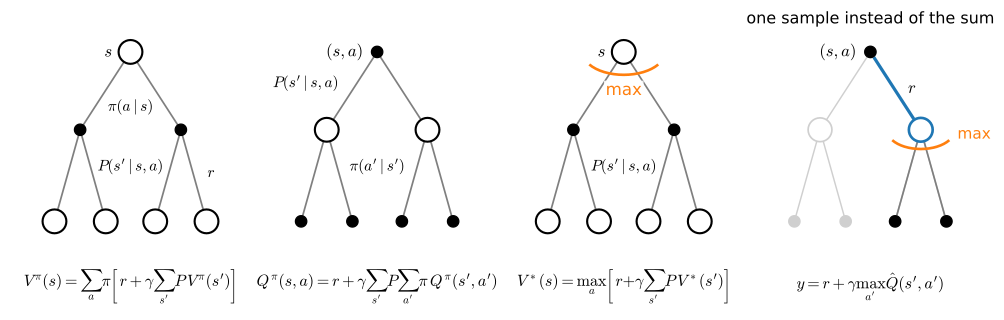
The four equations of this section share one shape: the value at a root is assembled from values one step below it. Updates of this kind are called backups, because they carry value backwards, from futures to presents; Figure 14.2.1 draws the vocabulary. Every algorithm in these two chapters walks one step down such a tree, and when Section 14.4 replaces the environment’s average by a single observed transition, the change is the one blue path through the rightmost diagram.
14.2.3 Convergence via Contraction
The Bellman optimality equation defines \(V^*\) implicitly. To compute it, read Equation 14.2.8 as a map: the Bellman optimality operator \(T\) acts on any table \(V: \mathcal{S} \to \mathbb{R}\) by
\[(TV)(s) = \max_{a \in \mathcal{A}} \Big[ r(s, a) + \gamma \sum_{s' \in \mathcal{S}} P(s' \mid s, a)\ V(s') \Big], \tag{14.2.10}\]
so that Equation 14.2.8 says exactly \(V^* = TV^*\): the optimal value function is a fixed point of \(T\), and \(T\) turns out to shrink distances.
14.2.3.1 The Contraction Proposition
Distance between value functions is measured in the sup norm \(\|V\|_\infty = \max_{s} |V(s)|\), the largest disagreement at any state.
Proposition (the Bellman operator is a \(\gamma\)-contraction). For any two tables \(V, V': \mathcal{S} \to \mathbb{R}\),
\[\|TV - TV'\|_\infty \leq \gamma\, \|V - V'\|_\infty. \tag{14.2.11}\]
Proof. Fix \(s\) and write \(f(a)\) and \(g(a)\) for the bracketed terms in \((TV)(s)\) and \((TV')(s)\). For every \(a\), \(|f(a) - g(a)| = \gamma\, |\sum_{s'} P(s' \mid s, a)(V(s') - V'(s'))| \leq \gamma \|V - V'\|_\infty\), because the probabilities are non-negative and sum to one. A maximum moves less than its inputs, \(|\max_a f(a) - \max_a g(a)| \leq \max_a |f(a) - g(a)|\), so \(|(TV)(s) - (TV')(s)| \leq \gamma \|V - V'\|_\infty\) for every \(s\). \(\blacksquare\)
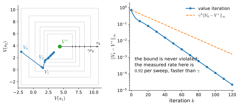
The discount that made the return finite in Section 14.1 here makes planning converge. This is precisely the situation of Banach’s fixed-point theorem, the tool that gave differential equations existence and uniqueness in Section 29.1.1.3, and the picture (Figure 14.2.2) is the same: nested balls closing in on a point the map cannot escape.
14.2.3.2 Four Consequences: Uniqueness, Rate, Stopping Rule and the \(\gamma = 1\) Boundary
Everything this chapter needs falls out in four steps. First, uniqueness: two fixed points would satisfy \(\|V - V'\|_\infty \leq \gamma \|V - V'\|_\infty\), which for \(\gamma < 1\) forces \(\|V - V'\|_\infty = 0\): the optimality equation pins \(V^*\) down completely. Second, convergence from anywhere, at rate \(\gamma\): iterating \(V_{k+1} = TV_k\) from any \(V_0\) gives
\[\|V_k - V^*\|_\infty = \|TV_{k-1} - TV^*\|_\infty \leq \gamma\, \|V_{k-1} - V^*\|_\infty \leq \cdots \leq \gamma^k\, \|V_0 - V^*\|_\infty, \tag{14.2.12}\]
so reaching accuracy \(\varepsilon\) takes at most \(\log(\|V_0 - V^*\|_\infty / \varepsilon) / \log(1/\gamma)\) sweeps; since \(\log(1/\gamma) \approx 1 - \gamma\) near one, that is the effective horizon \(1/(1-\gamma)\) of Section 14.1 times \(\ln(1/\varepsilon)\): far-sighted objectives are solvable, just proportionally slower. Third, a stopping rule: the bound above mentions the unknown \(V^*\), but telescoping \(\|V_k - V^*\|_\infty \leq \sum_{j \geq k} \|V_{j+1} - V_j\|_\infty\) and shrinking each summand by \(\gamma\) per step gives
\[\|V_k - V^*\|_\infty \leq \frac{\gamma}{1 - \gamma}\, \|V_k - V_{k-1}\|_\infty, \tag{14.2.13}\]
a certificate built from the observable sweep-to-sweep change, which is what an implementation should actually test; we do so below. Fourth, the boundary: at \(\gamma = 1\) the contraction modulus is \(1\), the argument collapses, and the undiscounted operator can have no fixed point or a continuum of them; episodic problems at \(\gamma = 1\) can still behave (ours does), but the guarantee is gone (exercise 5 makes both halves precise). Finally, the max entered the proof only through the “maximum of differences” step, so replacing it by an average under a fixed policy \(\pi\) yields an operator \(T^\pi\) that contracts by the same argument, with unique fixed point \(V^\pi\). One proof, two algorithms; the full theory is in (Puterman 1994; Bertsekas 2025).
14.2.4 Value Iteration, Policy Evaluation and Policy Iteration
A theorem this constructive is rare: its proof is an algorithm, and this section runs it on the slippery lake of Section 14.1, rebuilt as a dense model in two lines:
gamma = 0.95
LEFT, DOWN, RIGHT, UP = 0, 1, 2, 3
env = gym.make('FrozenLake-v1', is_slippery=True)
mdp = d2l.TabularMDP.from_gym(env, gamma)
gamma = 0.95
LEFT, DOWN, RIGHT, UP = 0, 1, 2, 3
env = gym.make('FrozenLake-v1', is_slippery=True)
mdp = d2l.TabularMDP.from_gym(env, gamma)14.2.4.1 Value Iteration
Iterate the operator: initialize \(V_0\) arbitrarily (we use zeros) and sweep
\[V_{k+1}(s) = \max_{a \in \mathcal{A}} \Big[ r(s, a) + \gamma\ \sum_{s' \in \mathcal{S}} P(s' \mid s, a)\ V_k(s') \Big];\ \textrm{for all } s \in \mathcal{S}, \tag{14.2.14}\]
that is, \(V_{k+1} = TV_k\). This is value iteration, and the contraction has already done the analysis: \(V_k \to V^*\) from any initialization, at rate \(\gamma\). In code the sweep is one line, because mdp.backup from Section 14.1 computes the bracket for every state-action pair at once:
def value_iteration(mdp, num_iters):
    """Sweep V <- max_a backup(V); return the whole history of iterates."""
    V, history = np.zeros(mdp.num_states), []
    for _ in range(num_iters):
        V = mdp.backup(V).max(axis=1)
        history.append(V)
    return np.array(history)
def value_iteration(mdp, num_iters):
"""Sweep V <- max_a backup(V); return the whole history of iterates."""
V, history = np.zeros(mdp.num_states), []
for _ in range(num_iters):
V = mdp.backup(V).max(axis=1)
history.append(V)
return np.array(history)Value iteration is the only algorithm in this book that plans with the model itself: everything from Section 14.4 onward touches only sampled transitions, because outside a simulator nobody hands you env.unwrapped.P. Keep this section in mind as the model-based corner of the map. We run it far past convergence, keep the final iterate as \(V^*\), and extract the policy by the greedy lookahead Equation 14.2.9:
history = value_iteration(mdp, num_iters=1000)
V_star = history[-1]
pi_star = mdp.backup(V_star).argmax(axis=1)
print(f'V*(s0) = {V_star[0]:.4f}')
d2l.show_grid(env.unwrapped.desc, V_star, pi_star)
V*(s0) = 0.1805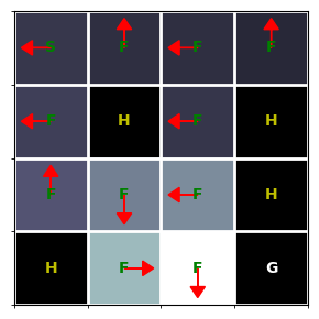
history = value_iteration(mdp, num_iters=1000)
V_star = history[-1]
pi_star = mdp.backup(V_star).argmax(axis=1)
print(f'V*(s0) = {V_star[0]:.4f}')
d2l.show_grid(env.unwrapped.desc, V_star, pi_star)
V*(s0) = 0.1805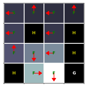
The values climb from about \(0.18\) at the start toward \(0.72\) beside the goal, and notice how modest they are: on calm ice the start would be worth \(\gamma^5 \approx 0.774\), so the slips destroy three quarters of its value even under optimal play. Several arrows point away from the goal; we defer reading them to the last subsection and first check the theory against the run:
err = np.concatenate([[np.abs(V_star).max()],
                      np.abs(history - V_star).max(axis=1)])
k = np.arange(131)
assert (err[k] <= err[0] * gamma ** k + 1e-12).all()
d2l.plot_curves({'value iteration': np.log10(err[k]),
                 'gamma^k guarantee': np.log10(err[0] * gamma ** k)},
                xlabel='sweep k', ylabel='log10 of sup-norm distance to V*')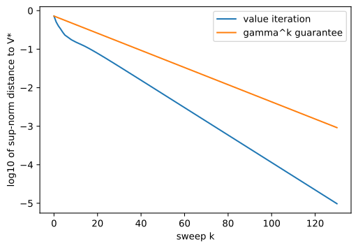
err = np.concatenate([[np.abs(V_star).max()],
                      np.abs(history - V_star).max(axis=1)])
k = np.arange(131)
assert (err[k] <= err[0] * gamma ** k + 1e-12).all()
d2l.plot_curves({'value iteration': np.log10(err[k]),
                 'gamma^k guarantee': np.log10(err[0] * gamma ** k)},
                xlabel='sweep k', ylabel='log10 of sup-norm distance to V*')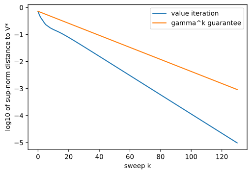
On this logarithmic scale geometric decay is a straight line, and the measured error hugs a line slightly steeper than the guaranteed one: the bound contracts by \(\gamma = 0.95\) per sweep, the run by about \(0.92\); the guarantee promises \(10^{-6}\) by sweep \(263\), the run gets there at \(158\). This is the correct mental model of the cost: the sweep count is set by the discount through the effective horizon, not by the size of the map, and not, on a stochastic problem, by the distance to the goal. An implementation, which cannot see the error curve, tests the stopping rule instead:
gap = np.abs(np.diff(history, axis=0)).max(axis=1)
true_err = np.abs(history[1:] - V_star).max(axis=1)
certified = gamma / (1 - gamma) * gap
assert (true_err <= certified + 1e-12).all()
for name, e in [('sweep-to-sweep change', gap),
                ('certified error bound', certified),
                ('distance to V*', true_err)]:
    print(f'{name} first below 1e-6 at sweep {np.argmax(e <= 1e-6) + 2}')
k_cert = np.argmax(certified <= 1e-6) + 2
sweep-to-sweep change first below 1e-6 at sweep 128
certified error bound first below 1e-6 at sweep 164
distance to V* first below 1e-6 at sweep 158gap = np.abs(np.diff(history, axis=0)).max(axis=1)
true_err = np.abs(history[1:] - V_star).max(axis=1)
certified = gamma / (1 - gamma) * gap
assert (true_err <= certified + 1e-12).all()
for name, e in [('sweep-to-sweep change', gap),
('certified error bound', certified),
('distance to V*', true_err)]:
print(f'{name} first below 1e-6 at sweep {np.argmax(e <= 1e-6) + 2}')
k_cert = np.argmax(certified <= 1e-6) + 2sweep-to-sweep change first below 1e-6 at sweep 128
certified error bound first below 1e-6 at sweep 164
distance to V* first below 1e-6 at sweep 158The naive test, “stop when a sweep changes nothing beyond \(10^{-6}\)”, fires at sweep \(128\) and promises nothing by itself. Multiplied by \(\gamma / (1 - \gamma) = 19\) it becomes a certificate, firing at sweep \(164\); the truth it certifies crossed \(10^{-6}\) at sweep \(158\). A guaranteed answer costs a handful of extra sweeps, and the assert confirms the certificate never lies.
14.2.4.2 Policy Evaluation
Replace the max in Equation 14.2.14 by the policy’s own average and the same iteration computes the value of any fixed policy \(\pi\):
\[V^\pi_{k+1}(s) = \sum_{a \in \mathcal{A}} \pi(a \mid s) \Big[ r(s, a) + \gamma\ \sum_{s' \in \mathcal{S}} P(s' \mid s, a)\ V^\pi_k(s') \Big];\ \textrm{for all } s \in \mathcal{S}. \tag{14.2.15}\]
This is policy evaluation, the fixed-point iteration for \(T^\pi\), convergent from any initialization because \(T^\pi\) contracts too. With the max gone the equations are linear, so they can also be solved directly, as Section 14.1 did with np.linalg.solve; the sweep does the same work one contraction at a time, and is the form that generalizes beyond tables.
def policy_evaluation(mdp, pi, num_iters):
    """Same sweep with the max replaced by an average under pi(a|s)."""
    V, history = np.zeros(mdp.num_states), []
    for _ in range(num_iters):
        V = (pi * mdp.backup(V)).sum(axis=1)
        history.append(V)
    return np.array(history)

uniform = np.ones((mdp.num_states, mdp.num_actions)) / mdp.num_actions
print(f'V(s0) for the uniformly random policy: '
      f'{policy_evaluation(mdp, uniform, 400)[-1][0]:.4f}')
V(s0) for the uniformly random policy: 0.0078def policy_evaluation(mdp, pi, num_iters):
"""Same sweep with the max replaced by an average under pi(a|s)."""
V, history = np.zeros(mdp.num_states), []
for _ in range(num_iters):
V = (pi * mdp.backup(V)).sum(axis=1)
history.append(V)
return np.array(history)
uniform = np.ones((mdp.num_states, mdp.num_actions)) / mdp.num_actions
print(f'V(s0) for the uniformly random policy: '
f'{policy_evaluation(mdp, uniform, 400)[-1][0]:.4f}')V(s0) for the uniformly random policy: 0.0078The uniformly random walker of Section 14.1 finished almost none of its episodes; it is worth \(0.0078\) at the start, about four percent of the optimum. Evaluation is measurement without improvement, and the critics of Section 15.1 will spend most of their capacity doing approximately what these seven lines do exactly.
14.2.4.3 Policy Iteration and Generalized Policy Iteration
Evaluation plus the greedy step Equation 14.2.9 suggests a different algorithm: evaluate the current policy fully, act greedily on its value function, repeat. For this to work, greedy improvement must actually improve; that is the chapter’s third short theorem.
Proposition (policy improvement). Let \(\pi\) be any policy and let \(\pi'\) be greedy with respect to \(V^\pi\), that is \(\pi'(s) = \mathrm{argmax}_a \big[ r(s, a) + \gamma \sum_{s'} P(s' \mid s, a) V^\pi(s') \big]\). Then \(V^{\pi'}(s) \geq V^\pi(s)\) at every state, and if equality holds everywhere then both policies are optimal.
Proof. Greediness says one step of \(\pi'\) is at least as good as one step of \(\pi\): \(T^{\pi'} V^\pi = T V^\pi \geq T^\pi V^\pi = V^\pi\). The operator \(T^{\pi'}\) is monotone (its coefficients are probabilities), so \(V^\pi \leq T^{\pi'} V^\pi \leq (T^{\pi'})^2 V^\pi \leq \cdots \to V^{\pi'}\), the limit being \(T^{\pi'}\)’s unique fixed point. If \(V^{\pi'} = V^\pi\), the first line reads \(TV^\pi = V^\pi\), so \(V^\pi\) solves the optimality equation and uniqueness finishes the job. \(\blacksquare\)
Each round of policy iteration therefore strictly improves the policy until it is optimal, and a finite MDP has finitely many deterministic policies, so termination is guaranteed (Puterman 1994). Four lines, plus a stopping check:
pi, num_outer = uniform, 0
while True:
    V = policy_evaluation(mdp, pi, 800)[-1]                # evaluate pi
    new = np.eye(mdp.num_actions)[mdp.backup(V).argmax(axis=1)]  # improve
    num_outer += 1
    if (new == pi).all():                                  # nothing changed
        break
    pi = new
assert np.abs(V - V_star).max() < 1e-12
pi, num_outer = uniform, 0
while True:
V = policy_evaluation(mdp, pi, 800)[-1] # evaluate pi
new = np.eye(mdp.num_actions)[mdp.backup(V).argmax(axis=1)] # improve
num_outer += 1
if (new == pi).all(): # nothing changed
break
pi = new
assert np.abs(V - V_star).max() < 1e-12The assert is the point: two different algorithms agree on \(V^*\) to twelve decimals, which is what “the fixed point is unique” looks like in a terminal. The bookkeeping is lopsided, though:
ok = [(mdp.backup(V).argmax(axis=1) == pi_star).all() for V in history]
print(f'policy iteration: {num_outer} rounds of evaluate-then-improve')
print(f'value iteration: certified at sweep {k_cert}')
print(f'its greedy policy already equals pi* from sweep '
      f'{np.argmax(ok) + 1} on')
policy iteration: 2 rounds of evaluate-then-improve
value iteration: certified at sweep 164
its greedy policy already equals pi* from sweep 14 onok = [(mdp.backup(V).argmax(axis=1) == pi_star).all() for V in history]
print(f'policy iteration: {num_outer} rounds of evaluate-then-improve')
print(f'value iteration: certified at sweep {k_cert}')
print(f'its greedy policy already equals pi* from sweep '
f'{np.argmax(ok) + 1} on')policy iteration: 2 rounds of evaluate-then-improve
value iteration: certified at sweep 164
its greedy policy already equals pi* from sweep 14 onPolicy iteration needed two rounds: greedy on the random walker’s values is already optimal on this small lake, and the second round merely confirms it. But each round hid \(800\) evaluation sweeps, so the like-for-like comparison is in Bellman backups, not rounds; exercise 6 does that accounting. The more interesting number is value iteration’s: its greedy policy stops changing at sweep \(14\), some \(150\) sweeps before the values are certified. Policies converge long before values do, because the argmax needs only the ranking of the actions, not the digits.
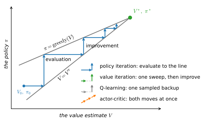
That observation licenses a whole design space: evaluation need not run to convergence before improvement acts, and improvement need not wait. Any interleaving that keeps nudging \(V\) toward \(V^\pi\) and \(\pi\) toward greedy(\(V\)) ends at the same corner, where both conditions hold and Equation 14.2.8 is satisfied. Sutton and Barto call this schema generalized policy iteration (GPI) (Sutton and Barto 2018), and Figure 14.2.3 draws it: policy iteration completes each move, value iteration improves after a single sweep, and the algorithms ahead take smaller, noisier steps still, Q-learning improving on one sampled backup (Section 14.4), actor-critic moving along both axes at once (Section 15.1). Whenever you wonder why acting greedily on a learned value estimate is sensible at all, the answer is the policy improvement theorem, applied with more or less patience.
14.2.4.4 The Optimal Policy on Slippery Ice
The theory certifies that \(\pi^*\) maximizes expected return; it does not say the result will look reasonable. Before reading the strange arrows, we need an instrument that scores a policy by average return over real episodes, the only standard that counts, with no access to the model:
def evaluate(env, policy, num_episodes, gamma=1.0, rng=None):
    """Mean discounted return of an acting policy over Monte Carlo episodes.

    `policy(obs, rng) -> action` is the protocol every agent in these two
    chapters speaks; a deterministic policy simply ignores `rng`."""
    total = 0.0
    for _ in range(num_episodes):
        obs, done, discount = env.reset()[0], False, 1.0
        while not done:
            obs, reward, terminated, truncated, _ = env.step(policy(obs, rng))
            done = terminated or truncated
            total, discount = total + discount * reward, discount * gamma
    return total / num_episodes
def evaluate(env, policy, num_episodes, gamma=1.0, rng=None):
"""Mean discounted return of an acting policy over Monte Carlo episodes.
`policy(obs, rng) -> action` is the protocol every agent in these two
chapters speaks; a deterministic policy simply ignores `rng`."""
total = 0.0
for _ in range(num_episodes):
obs, done, discount = env.reset()[0], False, 1.0
while not done:
obs, reward, terminated, truncated, _ = env.step(policy(obs, rng))
done = terminated or truncated
total, discount = total + discount * reward, discount * gamma
return total / num_episodesThe protocol matters: a policy is a function from observation to action, possibly consuming randomness from an explicit generator, and everything that acts in these two chapters will speak it. With the default \(\gamma = 1\) and terminal-only reward, the mean return is the success rate. Now pit \(\pi^*\) against the policy any of us would write first, the shortest path, as if the ice were calm:
shortest = np.array([DOWN, RIGHT, DOWN, LEFT,
                     DOWN, LEFT, DOWN, LEFT,
                     RIGHT, DOWN, DOWN, LEFT,
                     LEFT, RIGHT, RIGHT, LEFT])   # optimal on calm ice, by hand
env.reset(seed=0)
for name, p in [('slip-aware optimum', pi_star),
                ('shortest-path policy', shortest)]:
    success = evaluate(env, lambda s, _: int(p[s]), num_episodes=2000)
    print(f'{name}: reaches the goal in {success:.1%} of 2000 episodes')
slip-aware optimum: reaches the goal in 73.6% of 2000 episodes
shortest-path policy: reaches the goal in 4.7% of 2000 episodesshortest = np.array([DOWN, RIGHT, DOWN, LEFT,
DOWN, LEFT, DOWN, LEFT,
RIGHT, DOWN, DOWN, LEFT,
LEFT, RIGHT, RIGHT, LEFT]) # optimal on calm ice, by hand
env.reset(seed=0)
for name, p in [('slip-aware optimum', pi_star),
('shortest-path policy', shortest)]:
success = evaluate(env, lambda s, _: int(p[s]), num_episodes=2000)
print(f'{name}: reaches the goal in {success:.1%} of 2000 episodes')slip-aware optimum: reaches the goal in 73.6% of 2000 episodes
shortest-path policy: reaches the goal in 4.7% of 2000 episodesAbout \(0.74\) against about \(0.05\): the dynamic-programming policy reaches the goal roughly sixteen times as often. (The rates count episodes finishing within the environment’s \(100\)-step limit; a slip-aware walk is unhurried, and with the limit lifted its success probability is about \(0.78\).) The shortest path fails because five of its six moves are taken beside holes, and every command has two perpendicular slips; the optimum buys distance from the holes with time. Where it pays for safety is visible state by state:
row, col = np.arange(16) // 4, np.arange(16) % 4
to_row = np.clip(row + np.array([0, 1, 0, -1])[pi_star], 0, 3)
to_col = np.clip(col + np.array([-1, 0, 1, 0])[pi_star], 0, 3)
frozen = np.isin(env.unwrapped.desc.flatten(), [b'S', b'F'])
away = np.flatnonzero(frozen & ((3 - to_row) + (3 - to_col)
                                > (3 - row) + (3 - col)))
for s in away:
    print(f's={s:>2}: pi* commands {"<v>^"[pi_star[s]]}, '
          f'the shortest path takes {"<v>^"[shortest[s]]}')
s= 2: pi* commands <, the shortest path takes v
s= 6: pi* commands <, the shortest path takes v
s= 8: pi* commands ^, the shortest path takes >
s=10: pi* commands <, the shortest path takes vrow, col = np.arange(16) // 4, np.arange(16) % 4
to_row = np.clip(row + np.array([0, 1, 0, -1])[pi_star], 0, 3)
to_col = np.clip(col + np.array([-1, 0, 1, 0])[pi_star], 0, 3)
frozen = np.isin(env.unwrapped.desc.flatten(), [b'S', b'F'])
away = np.flatnonzero(frozen & ((3 - to_row) + (3 - to_col)
> (3 - row) + (3 - col)))
for s in away:
print(f's={s:>2}: pi* commands {"<v>^"[pi_star[s]]}, '
f'the shortest path takes {"<v>^"[shortest[s]]}')s= 2: pi* commands <, the shortest path takes v
s= 6: pi* commands <, the shortest path takes v
s= 8: pi* commands ^, the shortest path takes >
s=10: pi* commands <, the shortest path takes vAt four of the eleven frozen cells the optimal command moves the agent away from the goal, on the grid of Figure 14.1.1. One reads like a proof in miniature: at \(s = 8\), commanding up is the only action all three of whose outcomes avoid the hole at \(12\): slide left into the wall, slide right to \(9\), or move up to \(4\). The policy has also learned the wall trick: at \(s = 1\) and \(s = 3\) it commands up, straight into the wall, wasting the intended move so that only the harmless sideways slips remain. None of this is cleverness we put in; it is Equation 14.2.9 evaluating three-outcome averages nobody would compute by hand.
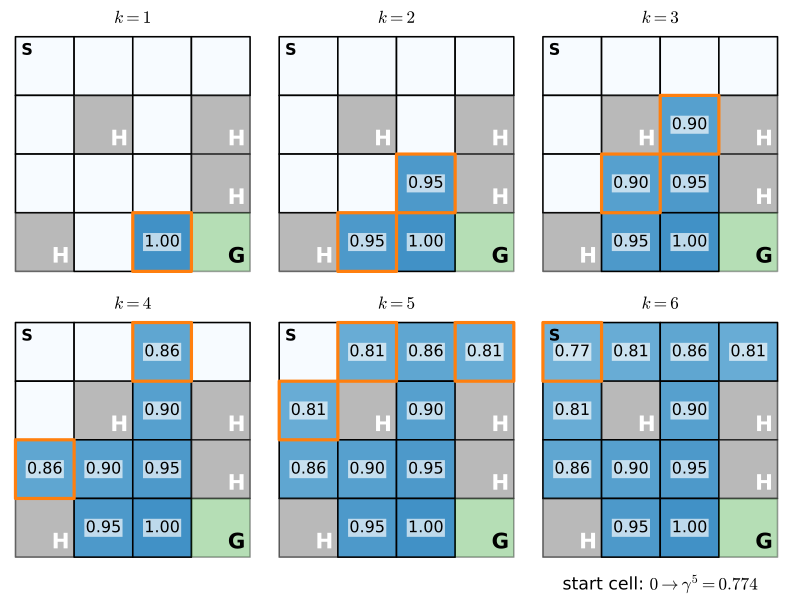
Aside: calm ice, in closed form. Switch the slip off and the subtlety vanishes so cleanly that the computation can be done in your head. With deterministic moves the optimality equation says \(V^*(s) = \gamma\, V^*(s')\) along the best move, so the value is \(\gamma^{d(s) - 1}\) with \(d(s)\) the number of moves to the goal, and sweep \(k\) reaches exactly the cells within \(k\) moves of it: convergence in six sweeps because the map is six moves deep (Figure 14.2.4). That wavefront reading of sweeps as steps to the goal holds only in this deterministic special case; on ice the sweep count is set by \(\gamma\), as we measured. The closed form also explains our hand-written opponent: greedy on the calm-ice solution is the shortest-path policy, which the assert below checks, so the \(0.05\) above is no strawman but the exact optimum of the wrong model.
calm = d2l.TabularMDP.from_gym(
    gym.make('FrozenLake-v1', is_slippery=False), gamma)
V_calm = value_iteration(calm, num_iters=10)[-1]
assert (calm.backup(V_calm).argmax(axis=1) == shortest).all()
print(f'V*(s0) on calm ice: {V_calm[0]:.4f};  gamma^5 = {gamma ** 5:.4f}')
V*(s0) on calm ice: 0.7738; gamma^5 = 0.7738calm = d2l.TabularMDP.from_gym(
gym.make('FrozenLake-v1', is_slippery=False), gamma)
V_calm = value_iteration(calm, num_iters=10)[-1]
assert (calm.backup(V_calm).argmax(axis=1) == shortest).all()
print(f'V*(s0) on calm ice: {V_calm[0]:.4f}; gamma^5 = {gamma ** 5:.4f}')V*(s0) on calm ice: 0.7738; gamma^5 = 0.7738The two start-state values bracket what the stochasticity costs, \(0.774\) calm against \(0.180\) on ice under optimal play: no policy can buy it back, only pay less of it than the shortest path does.
14.2.5 Summary
Given the model, acting well is computable. A policy is scored by \(V^\pi\) and \(Q^\pi\), linked by averaging, \(V^\pi(s) = \sum_a \pi(a \mid s) Q^\pi(s, a)\), with the advantage Equation 14.2.4 naming the gap improvement exploits. The Markov assumption folds infinite-horizon expectations into one-step recursions, the Bellman expectation equations for a fixed policy and the optimality equation Equation 14.2.8 for the best one. The optimality operator is a \(\gamma\)-contraction in the sup norm: its fixed point \(V^*\) is unique, value iteration converges geometrically from any start, and the sweep-to-sweep change certifies the error via the factor \(\gamma / (1 - \gamma)\). Policy evaluation is the same sweep without the max; policy iteration alternates it with greedy improvement, which provably never hurts; interleaving the two at any granularity is generalized policy iteration, the skeleton the coming learning algorithms hang on. All of it consumed env.unwrapped.P: this was the book’s one purely model-based section, and the measurement primitive evaluate is what survives when the model is taken away.
What the experiments show, and what they do not. Every number here except two is an exact computation on the known model, reproducible to the printed digit: the sweep counts (\(128\), \(158\), \(164\)), the start-state values (\(0.1805\) on ice, \(0.7738 = \gamma^5\) calm), the round count, and the away-pointing states are deterministic facts about one MDP at \(\gamma = 0.95\). The exceptions are the two Monte Carlo success rates, \(2{,}000\) seeded episodes each: rerunning with these seeds reproduces \(73.6\%\) and \(4.7\%\) exactly; a different seed moves each by a percentage point or so. The comparison shows that planning against the true stochastic model beats planning against a simplified one on this lake; it does not show how to act when the model is not given, which is the entire remaining problem of these two chapters.
14.2.6 Exercises
- [short-code] Cost of a sweep. Give the cost of one value iteration sweep Equation 14.2.14 in terms of the number of states, the number of actions, and the number of successors per state-action pair, and say which of the three the dense
mdp.backupof Section 14.1 actually pays for. Then use \(\|V_k - V^*\|_\infty \leq \gamma^k \|V_0 - V^*\|_\infty\) to show that reaching accuracy \(\varepsilon\) needs \(O(\log(1/\varepsilon) / \log(1/\gamma))\) sweeps. Confirm the per-sweep cost empirically (a few seconds) by timing the \(4 \times 4\) map against the \(8 \times 8\) map,d2l.TabularMDP.from_gym(gym.make('FrozenLake-v1', map_name='8x8', is_slippery=True), gamma). - [conceptual] The contraction, verified. The section’s proposition proved \(\|TV - TV'\|_\infty \leq \gamma \|V - V'\|_\infty\) using only that a maximum of differences bounds the difference of maxima. Re-derive the stopping rule \(\|V_k - V^*\|_\infty \leq \frac{\gamma}{1-\gamma} \|V_k - V_{k-1}\|_\infty\) from it by telescoping the tail \(\sum_{j \geq k} \|V_{j+1} - V_j\|_\infty\), and turn it into an \(\varepsilon\)-optimal stopping rule: how small must the sweep-to-sweep change be to guarantee an error below \(\varepsilon\)? Then walk through the proposition’s proof with \(\gamma = 1\) and point to the exact step that fails.
- [short-code] Predict, then run. Before running anything, predict \(V^*(s_0)\) on the calm map (
is_slippery=False) for \(\gamma \in \{0, 0.5, 0.9, 0.99\}\), and predict which of the four optimal policies differ. Now run value iteration for each and check. Explain in one sentence why the value depends on \(\gamma\) and the policy does not, and what is special about \(\gamma = 0\). - [short-code] Let the ice be calm. The section ran on slippery ice throughout. Switch the slip off, rerun value iteration, and compare the two optimal policies cell by cell. Which arrows change, and why does Equation 14.2.6 stop caring about the holes’ neighbors once \(P(s' \mid s, a)\) puts all its mass on the intended cell? The section printed \(V^*(s_0) = 0.180\) on ice and \(0.774\) calm, a ratio of about \(4.3\): is that larger or smaller than the naive reading “each commanded move now succeeds with probability \(1/3\)” suggests, and what does the difference say about what the optimal policy salvages from the slips?
- [conceptual] When \(\gamma\) equals one. The contraction proposition needs \(\gamma < 1\), yet running the section’s code with \(\gamma = 1\) on FrozenLake converges. Explain why, using that the goal and the holes are absorbing and all rewards are non-negative, and say what the limit \(V_k(s)\) means in that case. Then construct a two-state MDP with a single action on which \(V_k\) grows without bound at \(\gamma = 1\), and verify it in three lines of code.
- [extended] Policy iteration, charged in backups. Policy iteration converged in \(2\) rounds against value iteration’s \(164\) certified sweeps, which looks like a rout, but each round contained \(800\) evaluation sweeps of Equation 14.2.15 before the greedy step Equation 14.2.9. Charge both algorithms in the same currency, Bellman backups, and plot the sup-norm error against backups on the \(4 \times 4\) and \(8 \times 8\) maps (a few seconds each). Which converges in fewer outer iterations, which in fewer backups, and how does the answer move as \(\gamma \to 1\)? Does truncating the inner evaluation to ten sweeps change your accounting?