14 Reinforcement Learning
Every model in this book so far was trained and tested on data it did not choose. A classifier can be wrong about one image without changing which image arrives next: the test distribution is whatever the world serves, and the model’s outputs never touch it. An agent that acts has no such separation. Its output is an action, the action moves the world, and the next input is drawn from whatever state that action created, so the agent is the author of its own test distribution. One sentence carries the whole distinction: in standard deep learning the prediction of a trained model on one test datum does not affect the predictions on a future test datum; in reinforcement learning decisions at future instants (in RL, decisions are also called actions) are affected by what decisions were made in the past.
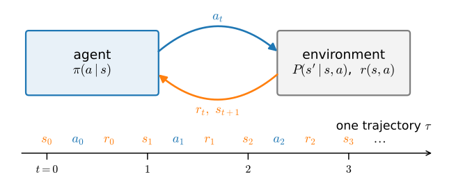
Everything distinctive about the subject is a consequence of that sentence. Data exists only where the agent goes, so gathering it becomes a decision with a price of its own. A small per-step error rate does not stay small, because one mistake moves every state that follows. An overvalued action summons exactly the data that convicts it, so acting on wrong estimates can be self-correcting, while an update taken too far can destroy the very distribution the agent must learn from next. We met distribution shift once before, in Section 3.7, as a misfortune that befalls a deployed model; here the model causes it, every time it acts. The stakes are immediate as well: a language model is a policy, its context a state and its vocabulary an action set, and the post-training that turns a base model into an assistant runs the estimators these two chapters build. Section 15.7 makes that correspondence exact, and the Language Models part puts it to work. The loop itself needs only one picture, Figure 14.1, and one identification worth fixing early: unroll the loop in time and its emissions are the data.
Seven sections build the subject in the order the difficulties arrive, and each closes with a measurement rather than a promise.
Section 14.1 builds the model of acting itself: the Markov decision process, four objects and one assumption, read out of a running simulator before being written in symbols. Three of the objects are facts about the world; the reward is authored, and an optimizer attacks the authorship. The section closes by paying a plausible bonus of \(0.3\) per step toward the goal and computing the policy this makes optimal: it turns away from the goal at the one cell bordering it and provably never finishes, worth \(2.15\) by the yardstick we wrote and exactly zero by the true one.
Section 14.2 hands the agent the model and solves it: the Bellman equations, an operator that contracts at rate \(\gamma\) and certifies its own stopping rule, and three algorithms from one proof. The payoff experiment is the chapter’s first surprise: on slippery ice the optimal policy is not the shortest path, reaching the goal \(0.74\) of the time against the shortest path’s \(0.05\) by buying distance from the holes with time, and commanding straight into walls so that only the harmless slips remain.
Section 14.3 throws the model away and copies an expert instead, a reduction to the softmax regression of Section 3.1. The clone makes zero mistakes on its 96 training pairs and still collapses from the expert’s \(73.4\) percent success to \(17.5\): it was certified on the expert’s states and is tested on the states its own actions create, a loss the section proves scales as \(\Theta(\varepsilon T^2)\) in the horizon. DAgger repairs it by changing nothing about the model and everything about where the data comes from, matching the expert on this small lake after one round of relabeling.
Section 14.4 removes the expert too. Replacing the expectation in the Bellman backup by the one transition the environment just produced gives the temporal-difference error and Q-learning, and grading the result against the locked-away truth shows five seeds recovering \(V^*\) to within \(0.006\) to \(0.021\), while the textbook step-size schedule \(1/(1+n)\) strands all five seeds below a seventh of the truth. Exploration then gets its own instrument, the bandit, and its own currency, regret: after 2000 pulls greedy has paid \(824\), fixed \(\epsilon\) has paid \(117\), and Thompson sampling \(32\).
Section 14.5 learns the policy directly: the log-derivative trick turns the gradient of the expected return into an average over the agent’s own rollouts, and the transition probabilities cancel out of it. Because sixteen states admit an exact gradient through a differentiable linear solve, the section measures what “unbiased” actually buys: the mean estimate’s cosine against the true gradient climbs from \(0.93\) to \(1.00\) as the batch grows, while a single batch-of-four estimate misses by more than three and a half times the gradient’s own length.
Section 14.6 reduces that noise without moving the mean. One zero-mean identity licenses reward-to-go, baselines and the control-variate optimum, and a hygiene pass separates look-alikes: centering is a baseline, dividing by \(\sigma\) is a step-size rescaling in disguise, and in the five-estimator race the normalized arm wins while taking steps about five times larger than those of the centered arm it otherwise equals, a confound the section prints beside the ranking. GRPO is the method behind recent reasoning language models, and its group-normalized weights are this section’s normalization, nothing more.
Section 14.7 swaps the table for a network and shows how little happens: a three-line diff moves the same training loop from the lake to CartPole, where every seed crosses \(400\) of the \(500\) ceiling within about fifty updates, and a Gaussian head carries the loop unchanged to continuous torques. What networks genuinely change is measured too: one update now moves every state at once, and the score-function and pathwise gradients of the same expectation differ in variance by a factor of about twenty. That gap is the estimator axis beneath the practical PPO-versus-SAC split, whose other axis is which data may drive the update.
The chapter after this one, Chapter 15, keeps the same laboratory and pays this chapter’s three debts: the agent built here learns only when episodes end (bootstrapping, Section 15.1), discards every batch after a single gradient step (safe reuse, Section 15.2, and replay, Section 15.4), and has no notion of how large a policy step is safe, which matters precisely because a policy generates its own future data. Its final section severs the loop entirely and learns from a fixed log (Section 15.6), where the sign of safe optimism flips. Figure 14.2 places both chapters on one map, organized by the two questions that sort every algorithm: what is learned, and which data may drive the update.
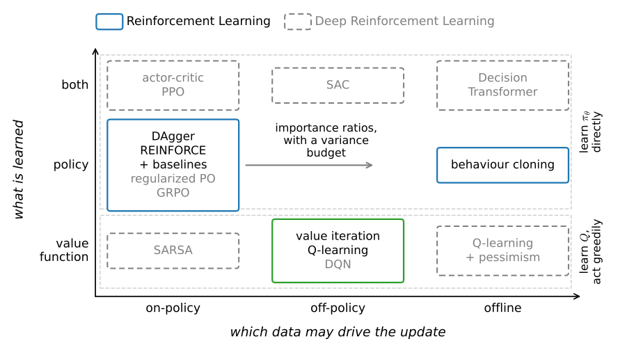
The map’s boxes hide a finer grain, and a first introduction owes the reader addresses for what it does not teach. Table 14.1 is the orientation table for both chapters: each algorithm, what it estimates, which data may drive its update, and where in this book it is taught or, failing that, named.
| algorithm | what it estimates | which data may drive the update | where |
|---|---|---|---|
| value iteration | \(V^*\) exactly, by sweeping the Bellman operator | none: it consumes the kernel \(P\) and reward \(r\) | Section 14.2 |
| behavior cloning | \(\pi(a \mid s)\) by cross-entropy on demonstrations | a fixed expert dataset | Section 14.3 |
| DAgger | the same fit | the learner’s own states, relabeled by an expert on call | Section 14.3 |
| Q-learning (tabular) | \(Q^*\) from sampled backups | any behavior’s transitions (off-policy) | Section 14.4 |
| SARSA | the behavior’s own \(Q\), exploration included | its own transitions (on-policy) | named in Section 14.4 |
| UCB, Thompson sampling | arm means plus their uncertainty | its own pulls (the bandit) | Section 14.4 |
| REINFORCE | \(\nabla_\theta J\) by the score function | fresh trajectories from the current policy only | Section 14.5 |
| REINFORCE with baselines, RLOO | the same gradient at lower variance | fresh trajectories from the current policy | Section 14.6 |
| GRPO | group-normalized advantages, no value network | fresh groups of responses per prompt | weights in Section 14.6; machinery in Chapter 15 |
| REINFORCE with a learned critic, on networks | \(\pi_\theta\) and \(\hat{V}\) as networks | fresh trajectories from the current policy | Section 14.7 |
| actor-critic (A2C) | \(\pi_\theta\) plus a bootstrapped critic | fresh, near-current trajectories | Section 15.1 |
| PPO | \(\pi_\theta\) under a clipped probability ratio | one batch, reused for a few steps | Section 15.2 |
| KL-regularized policy optimization, RLHF | a policy tilted from a reference by reward | rollouts scored by a learned reward | Chapter 15 |
| DQN, Double DQN | \(Q\) as a network | a replay buffer of stale experience | Section 15.4 |
| Rainbow | DQN plus its measured components | a replay buffer | named in Section 15.4 |
| DDPG, TD3 | a critic, and a deterministic actor trained to maximize it | a replay buffer (off-policy) | named in Section 14.7 and Section 15.5 |
| SAC | twin soft critics, and a stochastic squashed actor maximizing reward plus entropy | a replay buffer (off-policy) | Section 15.5 |
| offline Q-learning with pessimism, CQL | \(Q\) penalized where the data is thin | a fixed logged dataset, no interaction at all | Section 15.6 |
| Decision Transformer | a return-conditioned sequence model | a fixed logged dataset | named in Section 15.6 |
| MuZero, Dreamer | a learned model of the environment, to plan or imagine in | its own interaction, replayed through the model | named in Chapter 15 |
| DPO | the regularized optimum directly from preferences | a fixed preference dataset | Chapter 15 and the Language Models part |
Nearly everything above runs on one recipe: two environments, sixteen states and four numbers, a frozen lake read out as a transition table and a cart balancing a pole; every run in these two chapters takes seconds to a couple of minutes on a laptop CPU, and that is a design decision, not a limitation, because reinforcement-learning results are only readable across seeds and reruns, and the compute for those belongs to readers. Table 14.2 lists the headline experiments together with the thing every measurement in this field has: a confounder to hold in mind whenever a conclusion reads stronger than its table.
| experiment | what it probes | main confounder |
|---|---|---|
| the shaped-reward attack (Section 14.1) | the reward as an interface an optimizer will exploit | an existence proof at one bonus size: at \(0.1\) the exploit vanishes while the policy is still subtly distorted |
| slip-aware optimum vs. shortest path (Section 14.2) | planning against the true stochastic model vs. a simplified one | success rates count episodes within the 100-step limit; 2000 episodes resolve them to about a point |
| the perfect clone that fails (Section 14.3) | train-equals-test breaking when the agent authors its own test distribution | one deliberately unlucky three-episode draw; the ten-dataset sweep measures how typical it is |
| the chain simulation (Section 14.3) | the \(\varepsilon T^2\) vs. \(\varepsilon T\) rates of compounding error | both imitators are extreme cases by construction; real tasks live between the rates |
| Q-learning graded against \(V^*\), and the step-size race (Section 14.4) | whether sampled backups recover the exact answer, and which schedules survive a finite budget | the training curve plateaus at the behavior’s ceiling, not the policy’s; the schedule verdicts are budget-specific |
| the bandit regret race (Section 14.4) | what each exploration rule keeps paying for information it already has | UCB’s bonus scale is tuned; means over twenty runs hide heavy tails |
| the exact-gradient yardstick (Section 14.5, reused in Section 14.6) | unbiasedness and variance of policy-gradient estimators, measured rather than asserted | one frozen mid-training policy; the constants move with the freeze point |
| the five-estimator race (Section 14.6) | which variance reductions actually speed up training | at a fixed learning rate the race tracks effective step size at least as much as variance |
| the three-line diff (Section 14.7) | that the derivations never used the table | three seeds license levels and trends, never digits |
| score vs. pathwise gradients (Section 14.7) | the structural variance gap between two gradients of one expectation | the factor of twenty is specific to this critic, spread and offset; the direction and mechanism are not |
The table is not decoration. Reinforcement-learning curves are wide: within a single method, the slowest seed can need more than twice the updates of the fastest with nothing changed but the randomness, so every multi-seed number in these chapters is quoted as a range or a median, never a digit, and every experiment is small enough to rerun. When a comparison ahead surprises you, the intended response is not belief but a rerun on fresh seeds.
A word on what this chapter is not. It contains no multi-agent, meta-, hierarchical or goal-conditioned reinforcement learning; partial observability receives one paragraph in Section 14.1 and no machinery; no model-based agent is implemented, since Section 14.2 is the book’s model-based corner and search of the AlphaZero kind remains a pointer; and the RLHF pipeline, DPO’s derivation and the GRPO trick zoo belong to the Language Models part, which receives from these two chapters the objects it needs: the estimators, the regularized objective, and the reading of text generation as a decision process. What remains is the loop of Figure 14.1, met seven ways: an agent that must act well on the distribution its own actions create, and the measured question of what each level of knowledge is worth: a model, an expert, or samples alone.
Resources and Further Reading
Grouped by role: the books under the theory, the courses that teach it, the implementations to build from, and the record of what makes these methods work in practice. All are freely accessible online.
Textbooks
- Sutton and Barto, Reinforcement Learning: An Introduction (Sutton and Barto 2018) remains the field’s front door, and the field now carries the profession’s highest honor: Sutton and Barto received the 2024 Turing Award for building it.
- Szepesvári, Algorithms for Reinforcement Learning (Szepesvári 2010) states this chapter’s algorithms and their guarantees in under a hundred pages.
- Bertsekas, A Course in Reinforcement Learning (Bertsekas 2025) teaches the same material from the optimal-control side, where dynamic programming is the trunk and learning the branch.
- Agarwal, Jiang, Kakade, and Sun, Reinforcement Learning: Theory and Algorithms (Agarwal et al. 2019) supplies the sample-complexity rates this chapter states qualitatively.
- Lattimore and Szepesvári, Bandit Algorithms (Lattimore and Szepesvári 2020) is the full theory behind the exploration interlude of Section 14.4.
Courses
- Berkeley CS285: Deep Reinforcement Learning is the standard graduate treatment of the material these two chapters open.
- Stanford CS234: Reinforcement Learning is the course closest in scope to this chapter: foundations, exploration, and policy gradients with their guarantees.
- Stanford CS224R: Deep Reinforcement Learning covers the practice, imitation and offline methods included.
- CMU 10-703: Deep Reinforcement Learning and Control pairs the algorithms with control and physical embodiment.
- MIT 6.7920: Reinforcement Learning: Foundations and Methods develops the dynamic-programming spine of Section 14.2 at full depth.
Annotated implementations
- CleanRL (Huang, Rousslan F. J. Dossa, et al. 2022) publishes single-file, benchmarked implementations of the major deep reinforcement learning algorithms; the natural next step after Section 14.7.
- Stable-Baselines3 (Raffin et al. 2021) is the reliable library form of the same algorithms, with tuned hyperparameters in its accompanying zoo.
- Gymnasium (Towers et al. 2024) documents the environment interface every agent in these two chapters speaks.
The record
- Spinning Up in Deep RL (Achiam 2018) is a short curriculum from the score function to SAC, written to be read beside running code.
- The 37 Implementation Details of Proximal Policy Optimization (Huang, Rousslan Fernand Julien Dossa, et al. 2022) documents, one detail at a time, how much of reported performance lives in choices papers do not mention; the strongest published argument for the estimator hygiene of Section 14.6.