%matplotlib inline
from d2l import torch as d2l
import gymnasium as gym
import numpy as np
import torch14.5 Policy Gradient
Section 14.2 planned with the model, Section 14.3 copied an expert, and Section 14.4 learned action values from samples, always extracting the policy indirectly, through an argmax over a table. This section learns the policy directly: write \(\pi_\theta(a \mid s)\) as a differentiable function of parameters \(\theta\) and ascend the expected return \(J(\theta)\) by gradient steps (Williams 1992). One identity, the log-derivative trick, turns that gradient into an average over trajectories; inside the average the transition probabilities cancel; and what remains is a quantity the agent can compute from its own rollouts, no model and no value function required. The derivation is short, and the measurement comes after it: we run the estimator, then hold it against the exact gradient, which our sixteen-state lake lets us compute, and see what unbiased does and does not buy. The price is fresh trajectories for every update and noise that shrinks only as \(1/\sqrt{n}\), and it sets up Section 14.6.
%matplotlib inline
from d2l import jax as d2l
from flax import nnx
import gymnasium as gym
import jax
from jax import numpy as jnp
import numpy as np
14.5.1 Parameterizing the Policy
Our laboratory is the FrozenLake of Figure 14.1.1, with one deliberate change: the slip is off.
gamma = 0.95
env = gym.wrappers.TimeLimit(
    gym.make('FrozenLake-v1', is_slippery=False).env, max_episode_steps=10_000)
gamma = 0.95
env = gym.wrappers.TimeLimit(
gym.make('FrozenLake-v1', is_slippery=False).env, max_episode_steps=10_000)The determinism is an assumption, and it buys this section its subject: on ice a policy that is still mostly random reaches the goal so rarely that whole-trajectory credit assignment collects no signal at any budget a textbook would spend, and here the estimator is the subject while the environment is only scenery. The wrapper juggling is a second deliberate choice, about the horizon: gym.make normally caps FrozenLake episodes at 100 steps, and we strip that limit, keeping a 10,000-step cap only as a safety net. The objective this section differentiates is the return of complete episodes, and a time limit imposed for data collection would quietly change it: an episode cut at step 100 would enter the average as if its future were worth nothing, so the estimator would be unbiased for that truncated objective, not for the \(J(\theta)\) it is about to be graded against. Stripping the limit costs nothing here: a softmax policy keeps every action’s probability positive, a walk on this finite lake therefore reaches a hole or the goal with probability one, and quickly in practice (a hundred thousand episodes of the uniform starting policy produced none longer than 80 steps), so the safety cap is never hit. Section 14.4 measured what the stochasticity costs the value-based side; Section 14.6 stays on this same calm map, same horizon convention.
14.5.1.1 Softmax Preferences
To learn a policy by gradient ascent we must first write it as a differentiable function of parameters. We already own the object that does: ActorCritic.tabular from Section 14.3 keeps one free parameter \(\theta_{s,a}\) per state-action pair, a preference, in an embedding table, and turns the preferences at state \(s\) into a distribution with a softmax,
\[\pi_\theta(a \mid s) = \frac{e^{\theta_{s,a}}}{\sum_{a'} e^{\theta_{s,a'}}}. \tag{14.5.1}\]
This is the model of Section 3.1 with an image replaced by a state index, and it is deliberately the class that behavior cloning trained: this section builds no new policy machinery, and policy_step will reappear below with only its weights reinterpreted. Zero initialization starts the policy exactly uniform. Note what the preferences are not: nothing constrains \(\theta_{s,a}\) to approximate a value such as \(Q(s, a)\), and nothing will; they are free parameters whose only job is to place probability well.
14.5.1.2 The Score Function
The softmax is easy to differentiate. Since \(\log \pi_\theta(a \mid s) = \theta_{s,a} - \log \sum_{a'} e^{\theta_{s,a'}}\), the derivative with respect to the preference \(\theta_{s,b}\) of any action \(b\) at the same state is
\[\frac{\partial \log \pi_\theta(a \mid s)}{\partial \theta_{s,b}} = \mathbf{1}(b = a) - \pi_\theta(b \mid s), \tag{14.5.2}\]
and the derivative with respect to the preferences of every other state is zero. The quantity \(\nabla_\theta \log \pi_\theta(a \mid s)\) is called the score function, and it is the central object of this section. Read Equation 14.5.2 twice: it raises the preference of the action actually taken and lowers the others in proportion to their current probability, and it sums to zero over \(b\), so an update can only redistribute probability at a state, never inflate all of it (exercise 1). We do not hand-code the equation anywhere; autograd differentiates log_prob for us, so the useful thing a short check can do is verify it, at a generic table rather than at the too-symmetric uniform start:
rng = np.random.default_rng(0)
check = d2l.ActorCritic.tabular(16, 4)
with torch.no_grad():   # move to a generic table, off the uniform start
    check.policy.weight.copy_(torch.as_tensor(rng.standard_normal((16, 4))))
check.log_prob(torch.tensor([6]), torch.tensor([2])).backward()
probs = np.exp(check.log_prob_np(np.repeat(6, 4), np.arange(4)))
hand = np.zeros((16, 4), dtype=np.float32)
hand[6], hand[6, 2] = -probs, 1 - probs[2]
print(bool(torch.allclose(check.policy.weight.grad, torch.as_tensor(hand),
atol=1e-6)))Truerng = np.random.default_rng(0)
theta = jnp.asarray(rng.standard_normal((16, 4))) # a generic table
score = jax.grad(lambda th: jax.nn.log_softmax(th[6])[2])(theta)
hand = jnp.zeros_like(theta).at[6].set(-jax.nn.softmax(theta[6]))
hand = hand.at[6, 2].add(1.0)
print(bool(jnp.allclose(score, hand, atol=1e-6)))TrueBoth tabs confirm the identity from the same random table, each by its own mechanism: the pytorch tab backpropagates through the model’s log_prob and reads the gradient off the embedding table, while the jax tab differentiates the log-softmax as a pure function of the table. From here on, every qualitative claim about what REINFORCE does to the preferences reads directly off Equation 14.5.2.
14.5.1.3 The Case for Stochastic Policies
Section 14.2 proved that a deterministic optimal policy always exists, so why parameterize a stochastic one? Three reasons, in increasing order of importance. A stochastic policy explores as a side effect of acting: the softmax keeps every action’s probability positive, so no separate \(\epsilon\)-greedy mechanism needs bolting on, though positive support is not a visitation guarantee, since a probability can fall so low that no finite budget of rollouts samples the action again, which is exactly how the plateaus at the end of this section form. A deterministic policy is not usefully differentiable: as a function of \(\theta\), an argmax is piecewise constant, its gradient zero almost everywhere, while the softmax makes \(\pi_\theta\), and through it the objective, smooth. And it is the parameterization that scales: put a network under the same softmax and Equation 14.5.1 is unchanged (Section 14.7); let the state be a context and the actions a vocabulary and it is a language model’s next-token distribution, trained at scale by the very updates this section derives (Section 15.7).
14.5.2 The Policy Gradient
With a differentiable policy in hand, acting well becomes an optimization problem, and this section is one derivation run to its end.
14.5.2.1 An Optimization Problem over Trajectories
Imagine, as in Section 14.2, that the agent starts at a state \(s_0\) and takes actions from the policy \(\pi_\theta\) for \(T\) timesteps, producing a trajectory \(\tau = (s_0, a_0, r_0, s_1, a_1, r_1, \ldots, s_T)\) with return \(R(\tau) = \sum_{t=0}^{T-1} \gamma^t r(s_t, a_t)\). The probability of observing a particular trajectory \(\tau\) is the product of the probabilities of each action taken by the agent and each transition made by the environment,
\[P(\tau; \theta) = \prod_{t=0}^{T-1} \pi_\theta(a_t \mid s_t)\ P(s_{t+1} \mid s_t, a_t). \tag{14.5.3}\]
If the start state were drawn from the distribution \(\mu_0\) of Section 14.1, a factor \(\mu_0(s_0)\) would multiply this product; it does not depend on \(\theta\) and drops out of every gradient below, so we keep the start state fixed as in our gridworld. Hold on to \(\mu_0\) anyway: when the Language Models part treats text generation as a decision process, the distribution over prompts is exactly this factor (Section 15.7). Our objective is the average return over trajectories, viewed as a function of the policy parameters,
\[J(\theta) = E_{\tau \sim P(\cdot;\, \theta)} \Big[ R(\tau) \Big] = \sum_{\tau} R(\tau)\ P(\tau; \theta), \tag{14.5.4}\]
where the summation runs over all possible trajectories of length \(T\). The fixed \(T\) is a bookkeeping device: pad every episode that ends early with the absorbing terminal state of Section 14.1, at zero reward, and all trajectories share a common horizon while the padded steps change nothing below, their rewards being zero and their scores averaging to zero given the prefix (a fact Section 14.6 proves and then turns into a tool), so the code may keep only the recorded episode. Note that \(J(\theta) = V^{\pi_\theta}(s_0)\) in the notation of Section 14.2 (our lake, with the time limit stripped, is episodic: every trajectory reaches a terminal state with probability one, so for \(T\) past the episode’s length the finite sum agrees with the infinite-horizon return); the new point of view is that we can search for good parameters directly,
\[\max_\theta J(\theta) = \max_\theta \sum_{\tau} R(\tau)\ P(\tau; \theta).\]
The trajectory is about to become the unit of data for everything ahead, so we give it a data structure before differentiating anything. A Batch stores the transitions of many episodes as flat arrays plus the boundaries between episodes, and it records the terminated flag, never truncated: Section 14.1 drew that line once, and this container is where the whole chapter keeps it.
class Batch:
    """A flat batch of transitions, plus the episode boundaries."""
    def __init__(self, obs, act, rew, next_obs, term, ep_ends):
        self.obs, self.act, self.rew = obs, act, rew
        self.next_obs, self.term = next_obs, term
        self.ep_ends = ep_ends    # one past the last step of each episode

    def __len__(self):
        return len(self.rew)

    def episodes(self):
        """Yield one slice per episode."""
        start = 0
        for end in self.ep_ends:
            yield slice(start, end)
            start = end

    def episode_returns(self, gamma=1.0):
        """R(tau), the discounted return, one number per episode."""
        return np.array([(gamma ** np.arange(ep.stop - ep.start)
                          * self.rew[ep]).sum() for ep in self.episodes()])
class Batch:
"""A flat batch of transitions, plus the episode boundaries."""
def __init__(self, obs, act, rew, next_obs, term, ep_ends):
self.obs, self.act, self.rew = obs, act, rew
self.next_obs, self.term = next_obs, term
self.ep_ends = ep_ends # one past the last step of each episode
def __len__(self):
return len(self.rew)
def episodes(self):
"""Yield one slice per episode."""
start = 0
for end in self.ep_ends:
yield slice(start, end)
start = end
def episode_returns(self, gamma=1.0):
"""R(tau), the discounted return, one number per episode."""
return np.array([(gamma ** np.arange(ep.stop - ep.start)
* self.rew[ep]).sum() for ep in self.episodes()])Filling it is a loop over the evaluate protocol of Section 14.2, a policy being any function policy(obs, rng) -> action:
def rollout(env, policy, num_episodes, rng):
    """Collect complete episodes from `policy(obs, rng) -> action` as a
    Batch; `term` records `terminated`, never `truncated` (:numref:`sec_mdp`).

    All sampling runs through the one numpy generator `rng`."""
    cols, ep_ends = [[] for _ in range(5)], []
    for _ in range(num_episodes):
        obs, done = env.reset()[0], False
        while not done:
            act = policy(obs, rng)
            next_obs, reward, terminated, truncated, _ = env.step(act)
            done = terminated or truncated
            for col, val in zip(cols, (obs, act, reward, next_obs,
                                       float(terminated))):
                col.append(val)
            obs = next_obs
        ep_ends.append(len(cols[0]))
    obs, act, rew, next_obs, term = (np.asarray(c) for c in cols)
    return Batch(obs, act, rew.astype(np.float32), next_obs,
                 term.astype(np.float32), np.asarray(ep_ends))
def rollout(env, policy, num_episodes, rng):
"""Collect complete episodes from `policy(obs, rng) -> action` as a
Batch; `term` records `terminated`, never `truncated` (:numref:`sec_mdp`).
All sampling runs through the one numpy generator `rng`."""
cols, ep_ends = [[] for _ in range(5)], []
for _ in range(num_episodes):
obs, done = env.reset()[0], False
while not done:
act = policy(obs, rng)
next_obs, reward, terminated, truncated, _ = env.step(act)
done = terminated or truncated
for col, val in zip(cols, (obs, act, reward, next_obs,
float(terminated))):
col.append(val)
obs = next_obs
ep_ends.append(len(cols[0]))
obs, act, rew, next_obs, term = (np.asarray(c) for c in cols)
return Batch(obs, act, rew.astype(np.float32), next_obs,
term.astype(np.float32), np.asarray(ep_ends))Both objects are plain numpy and shared verbatim between the framework tabs; framework arrays appear only inside update functions, converted at their first line, so everything a batch carries is data by construction. Nothing here is specific to this section: rollout feeds every learning algorithm in the rest of these two chapters.
14.5.2.2 The Log-Derivative Trick
To maximize \(J(\theta)\) by gradient ascent we need its gradient. The return \(R(\tau)\) of a fixed trajectory does not depend on \(\theta\), only the probability of the trajectory does, so (the summation is finite, so we can exchange it with the gradient)
\[ \begin{aligned} \nabla_\theta J(\theta) &= \nabla_\theta \sum_\tau R(\tau)\ P(\tau; \theta) = \sum_\tau R(\tau)\ \nabla_\theta P(\tau; \theta) \\ &= \sum_\tau R(\tau)\ P(\tau; \theta)\ \frac{\nabla_\theta P(\tau; \theta)}{P(\tau; \theta)} \\ &= \sum_\tau P(\tau; \theta)\ R(\tau)\ \nabla_\theta \log P(\tau; \theta), \end{aligned} \]
where we multiplied and divided by \(P(\tau; \theta)\) and used the identity \(\nabla \log P = \nabla P / P\). This step, known as the log-derivative trick, is important because it turns the gradient back into an average over trajectories,
\[\nabla_\theta J(\theta) = E_{\tau \sim P(\cdot;\, \theta)} \Big[ R(\tau)\ \nabla_\theta \log P(\tau; \theta) \Big], \tag{14.5.5}\]
and averages over trajectories are exactly what the agent can estimate by sampling: it simply runs its current policy.
14.5.2.3 Cancellation of the Transition Probabilities
At first sight Equation 14.5.5 still seems to require the MDP, because \(P(\tau; \theta)\) in Equation 14.5.3 contains the transition function. But watch what happens when we take the logarithm of the product and differentiate:
\[ \begin{aligned} \nabla_\theta \log P(\tau; \theta) &= \nabla_\theta \Big[ \sum_{t=0}^{T-1} \log \pi_\theta(a_t \mid s_t) + \sum_{t=0}^{T-1} \log P(s_{t+1} \mid s_t, a_t) \Big] \\ &= \sum_{t=0}^{T-1} \nabla_\theta \log \pi_\theta(a_t \mid s_t). \end{aligned} \]
The transition probabilities do not depend on the policy parameters \(\theta\), so their gradient is zero and they vanish from the expression. Just as in Q-Learning, we have not cheated: the transition function still determines which trajectories the agent is likely to experience, but we never need to evaluate it; it enters only implicitly, through the sampled data.
14.5.2.4 The REINFORCE Estimator
We now approximate the expectation in Equation 14.5.5 with an empirical average. The agent runs its current policy \(\pi_\theta\) to collect \(n\) trajectories \(\tau_1, \ldots, \tau_n\) and computes
\[\hat{u} = \frac{1}{n} \sum_{i=1}^n R(\tau_i)\ \sum_{t=0}^{T-1} \nabla_\theta \log \pi_\theta(a_t^i \mid s_t^i), \tag{14.5.6}\]
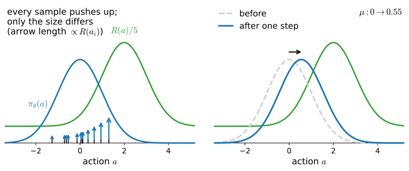
which is an unbiased estimate of \(\nabla_\theta J(\theta)\), and then takes a gradient ascent step \(\theta \leftarrow \theta + \alpha \hat{u}\) with learning rate \(\alpha\). This algorithm is known as REINFORCE (Williams 1992). It has a simple interpretation: each term pushes on the log-probability of the actions taken in trajectory \(\tau_i\), with that trajectory’s return as the coefficient. Read the direction with care: a sampled action’s own log-probability is pushed down only when its weight is negative, which cannot happen on this lake, where every return is \(0\) or positive. With all-positive weights every sampled action is pushed up, harder on better trajectories, and an action’s probability falls only through the softmax coupling, when competing samples at the same state are pushed harder; Section 14.6 constructs a weight with a meaningful zero point, positive for better than usual and negative for worse. Note that after every parameter update the policy changes, so the agent must collect fresh trajectories from the new policy before the next update. Figure 14.5.1 draws one such step on the smallest possible instance, every arrow pointing up and only the sizes sorting good actions from bad.
In code, the estimator is the policy_step of Section 14.3 with the weights finally carrying information: there every weight was \(1\), a teacher’s uniform endorsement; here the weight on every step of trajectory \(i\) is the return \(R(\tau_i)\) that whole trajectory earned. As with q_learning in Section 14.4, whatever the caller wants to keep is passed in, here the agent itself and a ledger of environment steps that the last part of this section will audit:
def train_reinforce(ac, seed, steps, num_updates=256, batch_episodes=16):
    """REINFORCE: a fresh batch from the current policy, every step of a
    trajectory weighted by that trajectory's return, one ascent step."""
    rng = np.random.default_rng(seed)      # one stream for all sampling
    env.reset(seed=seed)
    for _ in range(num_updates):
        batch = rollout(env, ac.act, batch_episodes, rng)
        R = batch.episode_returns(gamma)
        d2l.policy_step(ac, batch,
                        np.repeat(R, np.diff(batch.ep_ends, prepend=0)))
        steps.append(len(batch))
        yield float(R.mean())
def train_reinforce(ac, seed, steps, num_updates=256, batch_episodes=16):
"""REINFORCE: a fresh batch from the current policy, every step of a
trajectory weighted by that trajectory's return, one ascent step."""
rng = np.random.default_rng(seed) # one stream for all sampling
env.reset(seed=seed)
for _ in range(num_updates):
batch = rollout(env, ac.act, batch_episodes, rng)
R = batch.episode_returns(gamma)
d2l.policy_step(ac, batch,
np.repeat(R, np.diff(batch.ep_ends, prepend=0)))
steps.append(len(batch))
yield float(R.mean())One note on fidelity: Equation 14.5.6 sums each trajectory’s scores and divides by the number of trajectories \(n\), while policy_step averages over all steps in the batch. The two differ by a factor of the batch’s realized mean episode length, and that factor is random and correlated with how well the policy is doing, so the implemented update is a step-averaged variant of Equation 14.5.6, not the estimator the derivation covers: on any single batch the difference is a positive rescale of the same direction, but across batches it reweights them. We keep the variant because it is what practice runs, Section 14.6 measures all four divisor choices side by side, and the yardstick cells below compute Equation 14.5.6 itself, dividing by \(n\). Three seeds, and the curve each run yields is the estimate of \(J(\theta)\) itself, computed from the very trajectories that drove the updates, so it costs nothing extra:
agents, steps, curves = [], [], []
for seed in range(3):
    if tab.selected('pytorch'):
        torch.manual_seed(seed)            # init stream; the table is zeros
        agents.append(d2l.ActorCritic.tabular(16, 4))
    if tab.selected('jax'):
        agents.append(d2l.ActorCritic.tabular(16, 4, rngs=nnx.Rngs(seed)))
    steps.append([])
    curves.append(list(train_reinforce(agents[-1], seed, steps[-1])))
curves, steps = np.array(curves), np.array(steps)
d2l.plot_curves({'REINFORCE': curves}, xlabel='update',
                ylabel='mean return of the batch', reference=gamma ** 5)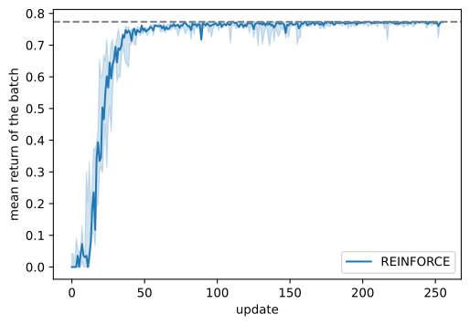
agents, steps, curves = [], [], []
for seed in range(3):
    if tab.selected('pytorch'):
        torch.manual_seed(seed)            # init stream; the table is zeros
        agents.append(d2l.ActorCritic.tabular(16, 4))
    if tab.selected('jax'):
        agents.append(d2l.ActorCritic.tabular(16, 4, rngs=nnx.Rngs(seed)))
    steps.append([])
    curves.append(list(train_reinforce(agents[-1], seed, steps[-1])))
curves, steps = np.array(curves), np.array(steps)
d2l.plot_curves({'REINFORCE': curves}, xlabel='update',
                ylabel='mean return of the batch', reference=gamma ** 5)
The curve has two phases. It hugs zero while success is an accident: a batch without a single successful trajectory has every \(R(\tau_i) = 0\), so Equation 14.5.6 is exactly zero and the policy does not move at all. Then improvement compounds, because every success sharpens the policy along its own path, which makes the next success likelier: within about thirty updates the batch mean crosses \(0.7\) and settles just below the dashed line at \(\gamma^5 \approx 0.774\), the return of a six-step path. It hovers below that ceiling because the policy stays stochastic: any sampled deviation from the path either lengthens the trajectory or ends it in a hole. What did it learn?
probs = np.exp(agents[0].log_prob_np(np.repeat(np.arange(16), 4),
                                     np.tile(np.arange(4), 16))).reshape(16, 4)
d2l.show_grid(env.unwrapped.desc, probs.max(axis=1), probs.argmax(axis=1))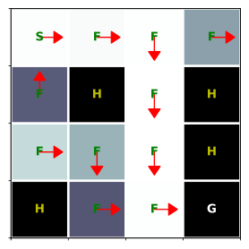
probs = np.exp(agents[0].log_prob_np(np.repeat(np.arange(16), 4),
                                     np.tile(np.arange(4), 16))).reshape(16, 4)
d2l.show_grid(env.unwrapped.desc, probs.max(axis=1), probs.argmax(axis=1))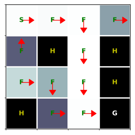
The arrows show each state’s most probable action and the shading its probability, from near-uniform (\(0.25\) with four actions) to near-certain. The policy has sharpened along a shortest path to the goal, though not necessarily the one value iteration produced for this calm map in Section 14.2: the grid admits three distinct six-step routes that avoid the holes, all of them optimal, and REINFORCE locks onto whichever one its first lucky trajectories happened to take, so a different seed can lock onto a different one. The cells that stay at exactly \(0.25\) are the holes and the goal: the agent never takes an action from a terminal state, so their preferences are never touched. The remaining cells are sharp in proportion to how often trajectories still visit them; states the converged policy no longer passes through stopped learning wherever they were.
14.5.2.5 The Policy Gradient Theorem
REINFORCE weights a whole trajectory’s score by the whole trajectory’s return. The same gradient has a second form, organized by states rather than by trajectories, which is how the literature most often writes it and how this book will use it from the next section on.
Proposition (policy gradient theorem). For the objective \(J(\theta) = E_{s_0 \sim \mu_0} [V^{\pi_\theta}(s_0)]\),
\[\nabla_\theta J(\theta) = E_{\tau \sim P(\cdot;\, \theta)} \Big[ \sum_{t \geq 0} \gamma^t\, \nabla_\theta \log \pi_\theta(a_t \mid s_t)\ Q^{\pi_\theta}(s_t, a_t) \Big] = \frac{1}{1 - \gamma}\, E_{s \sim d^{\pi_\theta}_\gamma,\ a \sim \pi_\theta(\cdot \mid s)} \Big[ \nabla_\theta \log \pi_\theta(a \mid s)\ Q^{\pi_\theta}(s, a) \Big], \tag{14.5.7}\]
where \(d^{\pi_\theta}_\gamma(s) = (1 - \gamma) \sum_{t \geq 0} \gamma^t \Pr(s_t = s)\) is the discounted state-occupancy distribution (Sutton et al. 2000).
Three readings. First, what multiplies the score at step \(t\) is no longer the whole trajectory’s return but the action value \(Q^{\pi_\theta}(s_t, a_t)\) of Section 14.2: rewards collected before step \(t\) cannot have been caused by the action taken there, and dropping them is the first variance reduction of Section 14.6. Second, the right-hand form averages over where the policy spends its discounted time rather than over trajectories; this is the form in which policy gradients meet theory, and the occupancy is where the start distribution \(\mu_0\) enters everything downstream. Third, a caveat that rarely gets a name: practical implementations sample states as visits accumulate, without the \(\gamma^t\) weights, which replaces the discounted occupancy \(d^{\pi_\theta}_\gamma\) by an undiscounted one. That is a change of state weighting, not merely of scale, so what they estimate is the gradient of a different objective than \(J\), with a direction of its own; nearly everyone drops the factor anyway, and exercise 6 prices the choice.
14.5.3 Costs and Limitations
14.5.3.1 The On-Policy Data Requirement
The estimator Equation 14.5.6 is an average over trajectories drawn from the current policy: it approximates Equation 14.5.5, an expectation under \(P(\tau; \theta)\). The moment the parameters move, trajectories collected earlier come from the wrong distribution, and the derivation licenses nothing about them. Methods with this property are called on-policy: the agent learns only about the policy it is executing, and every update pays for a fresh batch. Q-learning is the opposite kind, off-policy: the \(\max\) in its target lets it learn about the greedy policy from data collected by any policy (Section 14.4), so old experience keeps its value. The difference is not elegance but cost, and the ledger we kept prices it in the same currency as Section 14.4, environment steps:
hit = (curves >= 0.7).argmax(axis=1)
to_hit = np.array([s[:k + 1].sum() for s, k in zip(steps, hit)])
print(f'update at which the batch mean first reaches 0.7: {np.sort(hit)}')
print(f'environment steps spent by that update:  {np.sort(to_hit)}')
print(f'environment steps spent by the full run: {np.sort(steps.sum(axis=1))}')
update at which the batch mean first reaches 0.7: [24 27 30]
environment steps spent by that update: [3210 3789 4287]
environment steps spent by the full run: [26058 26582 27472]hit = (curves >= 0.7).argmax(axis=1)
to_hit = np.array([s[:k + 1].sum() for s, k in zip(steps, hit)])
print(f'update at which the batch mean first reaches 0.7: {np.sort(hit)}')
print(f'environment steps spent by that update: {np.sort(to_hit)}')
print(f'environment steps spent by the full run: {np.sort(steps.sum(axis=1))}')update at which the batch mean first reaches 0.7: [24 27 30]
environment steps spent by that update: [3210 3789 4287]
environment steps spent by the full run: [26058 26582 27472]The learning cost between three and four and a half thousand environment steps; the run cost about twenty-seven thousand, because an on-policy method keeps buying fresh data at the same rate after the policy has converged, and nothing it bought earlier can be reused. For scale, the median Q-learning run of Section 14.4 consumed \(95{,}569\) environment steps, though on the slippery map, where the task itself is harder; its deterministic contrast cell solved this same calm map from 256 episodes. The habit to keep is the bookkeeping itself: measure in environment steps, and remember that an on-policy bill scales with updates whether or not the updates still teach anything. Reusing a batch for several updates without correction is the obvious economy, and exercise 5 has you try it while watching the quantity that decides when it breaks, the probability ratio between the new policy and the one that collected the data; making that reuse safe is the subject of 1.
14.5.3.2 Unbiasedness and Variance
The word unbiased has been doing quiet work since Equation 14.5.6. It is a strong claim: the noisy vector computed from a handful of trajectories points, on average, exactly along \(\nabla_\theta J(\theta)\). Almost nobody ever checks it, because almost nobody has the true gradient; on sixteen states we do. For the softmax policy, writing \(P^\pi\) for its transition matrix and \(r^\pi\) for its expected one-step reward, the objective of Equation 14.5.4 has the closed form
\[J(\theta) = V^{\pi_\theta}(s_0) = \Big[ \big(I - \gamma P^{\pi_\theta}\big)^{-1} r^{\pi_\theta} \Big]_{s_0},\]
a linear solve, every step of it differentiable, so autograd delivers the exact \(\nabla_\theta J\) in milliseconds of CPU, the same trick of grading against locked-away truth as in Section 14.4. The interesting regime is mid-training, where the estimator still has work to do, so we freeze a fresh run after 16 updates:
mdp = d2l.TabularMDP.from_gym(env, gamma)
P, r = torch.as_tensor(mdp.P).float(), torch.as_tensor(mdp.r).float()
torch.manual_seed(3)
probe = d2l.ActorCritic.tabular(16, 4)
for _ in train_reinforce(probe, 3, [], num_updates=16):
    pass
theta = probe.policy.weight.detach().requires_grad_(True)
pi = torch.softmax(theta, -1)
J = torch.linalg.solve(torch.eye(16) - gamma * torch.einsum('sa,sat->st',
                                                            pi, P),
                       (pi * r).sum(-1))[0]
g_exact = torch.autograd.grad(J, theta)[0].numpy()
print(f'J(theta) after 16 updates = {J.item():.3f}, '
      f'against the ceiling gamma^5 = {gamma ** 5:.3f}')
J(theta) after 16 updates = 0.313, against the ceiling gamma^5 = 0.774mdp = d2l.TabularMDP.from_gym(env, gamma)
P, r = jnp.asarray(mdp.P), jnp.asarray(mdp.r)
probe = d2l.ActorCritic.tabular(16, 4, rngs=nnx.Rngs(3))
for _ in train_reinforce(probe, 3, [], num_updates=16):
pass
def J_fn(theta):
pi = jax.nn.softmax(theta, -1)
return jnp.linalg.solve(jnp.eye(16) - gamma * jnp.einsum('sa,sat->st',
pi, P),
(pi * r).sum(-1))[0]
theta = probe.policy.embedding[...]
g_exact = np.asarray(jax.grad(J_fn)(theta))
print(f'J(theta) after 16 updates = {float(J_fn(theta)):.3f}, '
f'against the ceiling gamma^5 = {gamma ** 5:.3f}')J(theta) after 16 updates = 0.313, against the ceiling gamma^5 = 0.774Now hold \(\theta\) fixed and draw the estimator Equation 14.5.6 fifty times at each batch size:
def reinforce_estimate(n, rng):
    """One draw of eq_reinforce: n fresh trajectories at the frozen theta."""
    batch = rollout(env, probe.act, n, rng)
    w = np.repeat(batch.episode_returns(gamma),
                  np.diff(batch.ep_ends, prepend=0)).astype(np.float32)
    th = probe.policy.weight.detach().requires_grad_(True)
    logp = torch.log_softmax(th, -1)[torch.as_tensor(batch.obs),
                                     torch.as_tensor(batch.act)]
    return torch.autograd.grad((torch.as_tensor(w) * logp).sum() / n,
                               th)[0].numpy().ravel()

rng, g = np.random.default_rng(4), g_exact.ravel()
for n in [4, 16, 64]:
    U = np.stack([reinforce_estimate(n, rng) for _ in range(50)])
    zero = int((np.linalg.norm(U, axis=1) == 0).sum())
    cos = U.mean(axis=0) @ g / (np.linalg.norm(U.mean(axis=0))
                                * np.linalg.norm(g))
    err = np.linalg.norm(U - g, axis=1).mean() / np.linalg.norm(g)
    print(f'n={n:>3}: zero estimates {zero:>2}/50, cos(mean, exact) = '
          f'{cos:.2f}, single-estimate relative error = {err:.2f}')
n= 4: zero estimates 3/50, cos(mean, exact) = 0.93, single-estimate relative error = 3.64
n= 16: zero estimates 0/50, cos(mean, exact) = 0.97, single-estimate relative error = 1.74
n= 64: zero estimates 0/50, cos(mean, exact) = 1.00, single-estimate relative error = 0.94def reinforce_estimate(n, rng):
"""One draw of eq_reinforce: n fresh trajectories at the frozen theta."""
batch = rollout(env, probe.act, n, rng)
w = jnp.asarray(np.repeat(batch.episode_returns(gamma),
np.diff(batch.ep_ends, prepend=0)))
def surrogate(th):
logp = jax.nn.log_softmax(th, -1)[batch.obs, batch.act]
return (w * logp).sum() / n
return np.asarray(jax.grad(surrogate)(theta)).ravel()
rng, g = np.random.default_rng(4), g_exact.ravel()
for n in [4, 16, 64]:
U = np.stack([reinforce_estimate(n, rng) for _ in range(50)])
zero = int((np.linalg.norm(U, axis=1) == 0).sum())
cos = U.mean(axis=0) @ g / (np.linalg.norm(U.mean(axis=0))
* np.linalg.norm(g))
err = np.linalg.norm(U - g, axis=1).mean() / np.linalg.norm(g)
print(f'n={n:>3}: zero estimates {zero:>2}/50, cos(mean, exact) = '
f'{cos:.2f}, single-estimate relative error = {err:.2f}')n= 4: zero estimates 3/50, cos(mean, exact) = 0.93, single-estimate relative error = 3.64
n= 16: zero estimates 0/50, cos(mean, exact) = 0.97, single-estimate relative error = 1.74
n= 64: zero estimates 0/50, cos(mean, exact) = 1.00, single-estimate relative error = 0.94Read the columns against the claim. The mean of the fifty estimates points essentially along the truth, its cosine with the exact gradient climbing from about \(0.93\) to \(1.00\) as \(n\) grows: that is what unbiasedness predicts, measured. The cosine is a diagnostic, not a proof, blind to length and to any error component parallel to the truth, so read it as consistency with the claim the derivation established. A single estimate is another matter. At \(n = 4\) its typical error is more than three and a half times the size of the gradient it estimates, and a few of the fifty batches contain no success at all, making their estimate exactly zero, a vector with no direction; the sparse reward is not just slow, it is degenerate (exercise 4). The error shrinks like \(1/\sqrt{n}\), roughly halving each time the batch quadruples, about \(3.6\) to \(1.7\) to \(0.9\) here, so brute force buys accuracy at quadratic cost in trajectories. These two cells are the chapter’s yardstick: Section 14.6 will change what multiplies the score, claim each change lowers the variance without moving the mean, and measure every such claim against this same exact gradient.
14.5.3.3 Nonconcavity of the Objective
One more limitation before summing up. Gradient ascent converged here, but nothing guarantees it in general, because \(J(\theta)\) is not a concave function of \(\theta\). The softmax makes \(J\) smooth, not concave: a policy that is nearly deterministic and wrong sits on a plateau where every probability in Equation 14.5.2 is close to \(0\) or \(1\), the scores and with them the whole gradient are vanishingly small, and ascent can spend arbitrarily long escaping. What the theory promises is a stationary point, under conditions our implementation does not check: smoothness, bounded estimator variance, Robbins-Monro step sizes rather than Adam at a fixed rate. That REINFORCE found an optimal policy every time here is a fact about a sixteen-state lake started from the maximum-entropy table, not an instance of a convergence theorem, and it is why the uniform start is the sensible default.
14.5.4 Summary
Policy gradient methods learn the policy directly: Equation 14.5.1 puts a softmax over free per-state preferences, reusing the ActorCritic container of Section 14.3, and the parameters ascend the expected return \(J(\theta)\). The log-derivative trick turns \(\nabla_\theta J\) into an expectation over trajectories Equation 14.5.5, the transition probabilities drop out of the score, so the method needs no model, and the empirical average is REINFORCE Equation 14.5.6: push up the log-probability of every action on a trajectory in proportion to that trajectory’s return. The policy gradient theorem restates the same gradient state by state, \(Q^{\pi_\theta}\) against the score under the discounted occupancy, the form the rest of the book builds on. The estimator is unbiased, which we measured against the exact \(\nabla_\theta J\) that a differentiable linear solve provides; it is noisy, its single-draw error shrinking only as \(1/\sqrt{n}\); and it is on-policy, so every update consumed a fresh batch whether or not it still had anything to learn. Two shared objects joined the library, Batch and rollout, the data path for every algorithm ahead.
What the experiments show, and what they do not. Every run is seeded, and all sampling in both framework tabs flows through the same shared numpy stream, so any divergence between the tabs can come only from the policies’ float32 probabilities, never from the data path; on this small table the two frameworks’ arithmetic stayed close enough that the printed numbers coincide at capture time, a coincidence the design does not promise, which is why the prose quotes rounded values. The training result (three seeds reaching the \(\gamma^5\) ceiling within about thirty updates for three to four and a half thousand environment steps) is specific to the calm map, named at the top of this section as a bought assumption: on ice this estimator at this budget learns nothing, and the fix is the next section’s subject. The yardstick numbers are one frozen mid-training policy probed with fifty draws per batch size; they demonstrate unbiasedness and the \(1/\sqrt{n}\) law, not the constants, which depend on where training was frozen. The cost comparison against Section 14.4 quotes that section’s printed number and flags the map mismatch rather than pretending it away. Single runs per configuration throughout: the compute belongs to readers.
14.5.5 Exercises
- [conceptual] The score sums to zero. Show that the derivative Equation 14.5.2 sums to zero over \(b \in \mathcal{A}\). Conclude that one REINFORCE update at a visited state can only redistribute probability among the actions at that state, never raise all of them. Which line of the section’s gradient-check cell encodes this identity, and what would break if the \(-\pi_\theta(b \mid s)\) term were dropped?
- [short-code] Unbiased, where enumeration is exact. Build a two-state, two-action MDP with horizon \(T = 2\), small enough to enumerate every trajectory. Repeat the yardstick measurement there: compute \(\nabla_\theta J(\theta)\) exactly from the sum in Equation 14.5.4, then compute the REINFORCE estimate Equation 14.5.6 from \(n \in \{10, 100, 10000\}\) sampled trajectories, ten times each, and plot the mean error and the standard deviation of the estimate against \(n\). Confirm the \(1/\sqrt{n}\) rate. Which of the two numbers does not shrink with \(n\) at all, and why is that the point?
- [short-code] Batch size and learning rate. Sweep
batch_episodesover \(\{1, 4, 16, 64\}\) and the learning rate ofActorCritic.tabularover \(\{0.03, 0.1, 0.3\}\), three seeds each, and report for every cell of the grid the total number of episodes (not updates) consumed before the batch mean return first exceeds \(0.5\). Which direction of the grid is a real improvement, and which merely trades updates for episodes? - [conceptual] Sparse reward, seen from the estimator. A trajectory that never reaches the goal has \(R(\tau) = 0\) and drops out of Equation 14.5.6 entirely. Now change the reward to \(-1\) per step with \(0\) at the goal, which encodes the same preference for short successful paths. Does the drop-out problem disappear? Describe the new pathology, and say which of the two reward conventions the baseline of Section 14.6 repairs.
- [short-code] Breaking the on-policy rule on purpose. Modify
train_reinforceto reuse each batch for \(k\) gradient steps without any correction, for \(k \in \{1, 2, 5, 20\}\). Alongside the return, log the mean and the maximum over the batch of \(\pi_\theta(a_t \mid s_t) / \pi_{\theta_{\textrm{old}}}(a_t \mid s_t)\) at the last of the \(k\) steps (log_prob_npmakes this two lines). At which \(k\) does the return start to suffer, and what is the ratio doing at that point? Keep the diagnostic in mind: it is the central object of - [conceptual] The discount that implementations drop. The trajectory form of the policy gradient theorem places a factor \(\gamma^t\) in front of the score at step \(t\). Weighting each step’s score by the reward-to-go without that factor, as the next section will, therefore estimates the gradient of a different objective. Write that objective down, say how it differs from \(J(\theta)\), and give a practical reason why nearly every implementation makes this choice anyway.